Here in Vancouver, the parking bylaw requires one 14m² parking space for every 20m² of supermarket floor space. Adding the necessary lanes to allow cars to get in and out, this law practically guarantees that grocery stores will be more parking lot than store.
In the late ’60s, the government sought to adopt O Canada as the national anthem. The music and original French lyrics had passed into the public domain, but the English version was still under copyright. The government settled the rights for a dollar.
Ironically, the copyright to the English lyrics would have expired anyways by the time the National Anthem Act was finally passed in 1980.
Crayola has a trademark on the smell of its crayons. The odour is described in the Canadian trademarks registry as:
A unique scent of a pungent, aldehydic fragrance combined with the faint scent of a hydrocarbon wax and an earthy clay.
In Canada, a trademark can be anything that is used by by a seller to distinguish their goods or services from those of others, including
a word, a personal name, a design, a letter, a numeral, a colour, a figurative element, a three-dimensional shape, a hologram, a moving image, a mode of packaging goods, a sound, a scent, a taste, a texture and the positioning of a sign.
Unfortunately, I have not been able to find records of anyone litigating over a scent trademark.
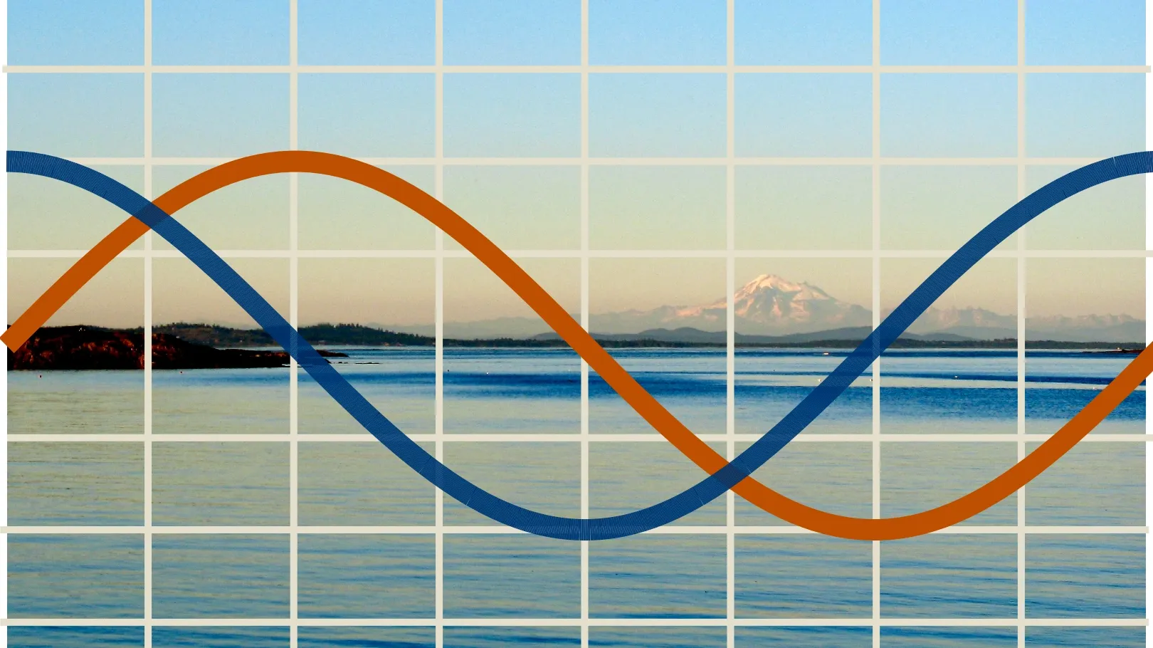
You can get a really good approximation of a sinusoidal curve from twelve equally-spaced line segments of slope 1/12, 2/12, 3/12, 3/12, 2/12, 1/12, -1/12, -2/12, -3/12, -3/12, -2/12, and -1/12, respectively.
This approximation, known as the rule of twelfths, rounds 3≈5/3 but otherwise uses exact values along the curve.
The rule of twelfths approximates points on (1−cos(2πx))/2.
I learned about the rule of twelfths from a kayaking instructor and guide, who used it to estimate the tides. In locations and seasons with a semidiurnal tide pattern, the period of the tide is roughly 12 hours, and the rule of twelfths tells you what the water will be doing in each hour.
For example, if you know that the difference between low and high tide is 3 feet, then you can quickly estimate that it the tide will rise by about 3 inches in the first hour, 6 inches in the second, 9 inches in the third and fourth, 6 inches in the fifth hour, and 3 inches in the last hour before high tide.
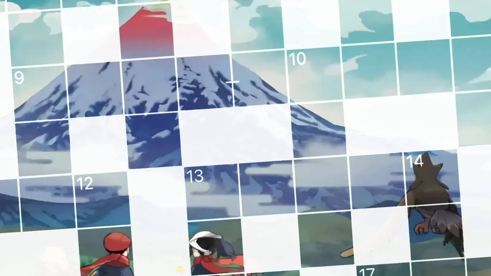
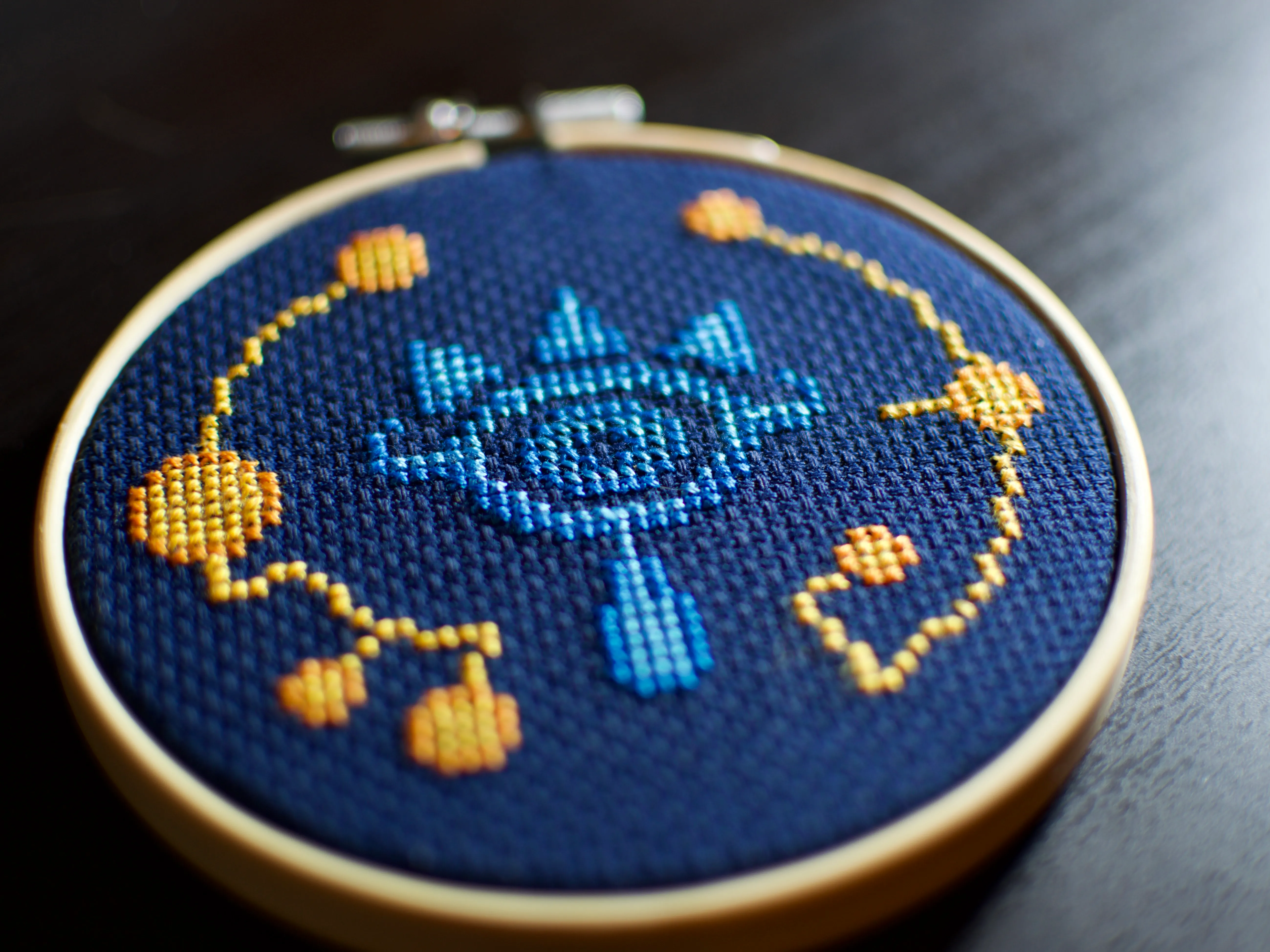
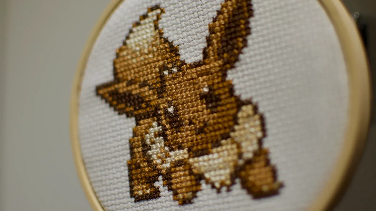
Recently I’ve been spending my spare time doing two things: solving cryptic crosswords and playing Pokémon Legends: Arceus. The next logical step, then, is to try my hand at compiling my own cryptic crossword themed after the game!
If you haven’t tried one before, a cryptic crossword is a crossword puzzle in which each clue is itself a word puzzle. A cryptic clue is usually misleading if taken at face value, but conceals a definition and a secondary indication (usually wordplay) of the correct answer. For example:
A gym leader in Cinnabar was inflamed (5)
The answer is RAGED, meaning “was inflamed”.
At first reading, it seems like this clue refers to the fiery Cinnabar Island Gym Leader Blaine from Pokémon Red and Blue, but the hidden real definition is only the last two words, “was inflamed”.
The remainder of the clue is wordplay that hints at the answer: “Cinnabar” means RED and “gym leader” can be interpreted as “the first letter of gym”, so “A gym leader in Cinnabar” reduces to “A G in RED” — hence, RAGED.
Cryptic clues can be even more complicated and include anagrams, homophones, obscure abbreviations, and all sorts of other devices. Or they can be as simple as a bad pun.
Feet passed down through generations? (7)
The answer is LEGENDS, which are “passed down through generations”. What
do feet have to do with anything? Well, they’re LEG ENDS, of course…
You’ll need to be a Pokémon fan to appreciate all of the surface readings in this puzzle, but don’t worry if you aren’t — none of the clues require any specific knowledge of Pokémon to solve. Once you’re done, you can scroll to the bottom to check the solutions and see how you did. Enjoy!
ACROSS
DOWN
Confused? Impatient? In the spirit of Fifteensquared, below is the answer key to the puzzle!
As a reminder, a cryptic clue generally consists of a dictionary definition and a secondary indication (usually wordplay) of the correct answer. In the following solutions, I’ve highlighted the dictionary definition hidden in each clue in bold.
Solution
Clue
RAGED
A gym leader in Cinnabar was inflamed (5)
I’ll then explain how the rest of the clue leads to the right answer, as well as how each clue relates to the puzzle theme.
Across
7 Across
Solution
Clue
BARBELL
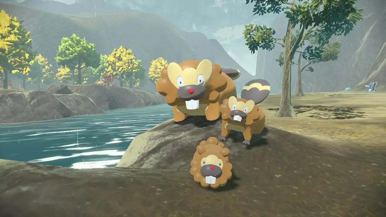
Angry Bibarel destroyed one-pound weight (7)
An anagram of BIBAREL after removing the letter I (“destroyed one”), plus L (“pound”). The anagram indicator is “angry”.
Received draught intended for negative condition (7)
A homophone of ale meant (“draught intended”). The homophone indicator is “received”.
The surface reading suggests an item like a Full Restore used in the Pokémon games to cure status conditions. The British spelling of draught/draft is partly in service of the surface reading; the influence of Harry Potter has made it more common in Canadian and American English when referring to potions and elixirs like those used in Pokémon.
9 Across
Solution
Clue
GOOD-NATURED
Jolly well suited ultimately to go after flora and fauna (4-7)
Breaks down into GOOD (“well”), and D (“suited ultimately”, meaning the last letter of suited) after NATURE (“flora and fauna”).
Natures in Pokémon are characteristics that increase one stat at the expense of another stat. “Jolly” is a good nature to have for certain Pokémon on a competitive team.
11 Across
Solution
Clue
KIND
Type disadvantage primarily follows lineage (4)
The letter D (“disadvantage primarily”, meaning the first letter of disadvantage) following KIN (“lineage”).
Pokémon types have strengths and weaknesses against each other; for example water-types are good against fire-types and ground-types are not effective against flying-types. Because Pokémon evolutionary lineages tend to share types, they also tend to share their type advantages and disadvantages.
The surface reading suggests Mount Coronet, the dominant geographical feature of Hisui. The answer references Alpha Pokémon, larger- and stronger-than-normal Pokémon that serve as minibosses in Pokémon Legends: Arceus.
Similar puns are present in Pokémon Legends: Arceus, as the items Grit Dust, Grit Gravel, Grit Pebble, and Grit Rock are used to raise Pokémon’s effort levels in a given stat.
16 Across
Solution
Clue
NOTCHES
Cuts tumblestone to catch child? (7)
An anagram of STONE surrounding (“catching”) the letters CH (abbreviating “child”). The anagram indicator is “tumble” although, as the question mark acknowledges, it’s slightly dubious to need to split apart a compound word in a cryptic clue.
A tumblestone is a raw material used when crafting Poké Balls to catch Pokémon with.
17 Across
Solution
Clue
AMNESIA
Memory loss means a name is confused (7)
An anagram of A NAME IS. The anagram indicator is “confused”.
The character Ingo in Pokémon Legends: Arceus suffers from amnesia after being transported through time and space from the Unova region.
19 Across
Solution
Clue
WARY
Cautious of battle decision (4)
A charade of WAR (“battle”) and Y (abbreviating yes, a “decision”).
Trainer battles in Pokémon Legends: Arceus end with a stylized wordmark reading “Battle decided”.
21 Across
Solution
Clue
START
Spookiest artifact conceals origin (5)
Concealed in spookieST ARTifact.
Three artifacts — the Adamant Crystal, Lustrous Globe, and Griseous Core — are used to change the legendary Pokémon Dialga, Palkia, and Giratina into their Origin Formes. Of these, the one associated with the Ghost-type Giratina is probably the spookiest.
22 Across
Solution
Clue
EPEE
Sword repeats point about Pokémon starter (4)
The letter E (“point”, as in the compass point east) repeated three times on either side of (“about”) P (“Pokémon starter”, meaning the first letter of Pokémon).
26 Across
Solution
Clue
CRYSTAL BALL
Lustrous Globe (7,4)
Cryptic definition — “Lustrous Globe” is just a funny way of saying “crystal ball”.
As mentioned above, the Lustrous Globe is a key item associated with the legendary Pokémon Palkia.
29 Across
Solution
Clue
EDITION
Version exclusives? To begin with, supplement lacks announcement (7)
The letter E (“exclusive to begin with”, meaning the first letter of exclusive), then ADDITION (“supplement”) lacking the first two letters AD (meaning “announcement”).
Historically, Pokémon games have been released in groups of slightly different versions, such as Pokémon Red and Blue, Pokémon Gold and Silver, and Pokémon Diamond and Pearl. The primary difference between versions in the same generation are Pokémon that can be caught in one game but not the other; these Pokémon are referred to as version exclusives. Pokémon Legends: Arceus is somewhat unique in that it is not paired with a second version (or supplementary DLC), so there are no version exclusives getting in the way of catching ‘em all.
30 Across
Solution
Clue
PHONIER
Phione evolution rumour: tip is more fraudulent (7)
An anagram of PHIONE, then R (“rumour tip” meaning the first letter of rumour). The anagram indicator is “evolution”.
Phione is a semi-mythical Pokémon which can be bred from, but strangely does not evolve into, Manaphy. False rumours and urban legends were common in the early days of Pokémon before reliable and comprehensive sources of information developed on the internet.
Down
1 Down
Solution
Clue
ARAGON
A dragon without a leader makes historic country (6)
The letter “A” is directly lifted from the clue, then DRAGON minus the first letter (“without a leader”). Aragon was a medieval kingdom that unified with Castile to form modern Spain.
Pokémon Legends: Arceus takes place in Hisui, a region loosely based on 19th-century Hokkaido. According to in-game legend, it was created by Arceus alongside the deities of time and space — which are revealed to actually be powerful Dragon-type Pokémon.
2 Down
Solution
Clue
RECON
Another trick for gathering information? (5)
Pun — if a trick is a con, is the second time you do it a re-con?
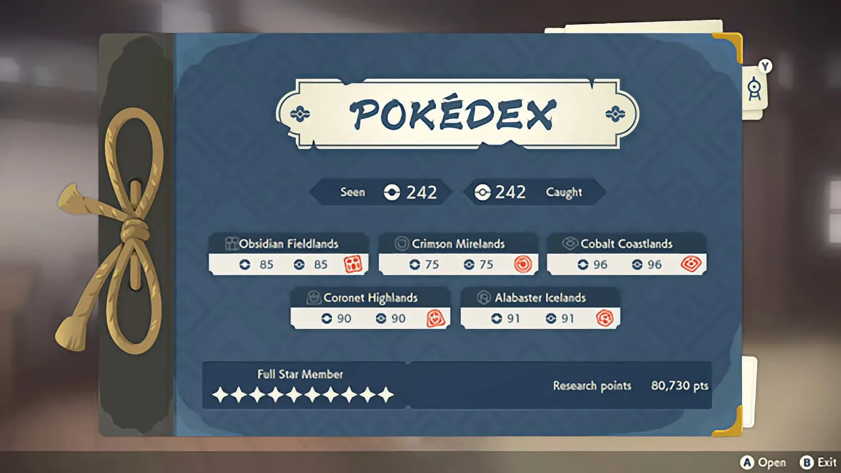
The ultimate goal of Pokémon Legends: Arceus is to perform research tasks to collect information on all the Pokémon, which are compiled into the Pokédex.
3 Down
Solution
Clue
CLAN
Family heads to calm lightning-affected nobles (4)
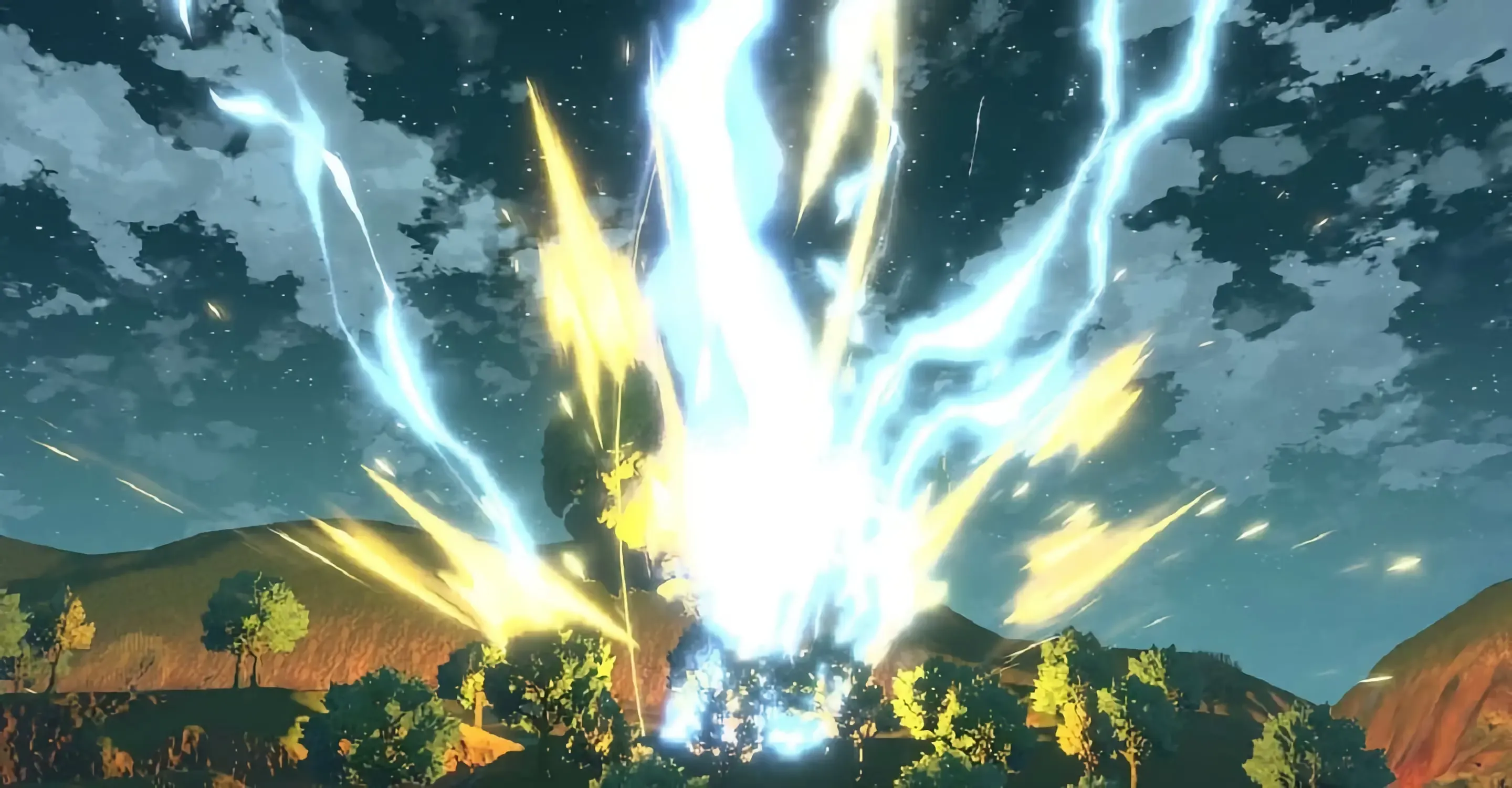
Formed from the first letters of (“heads to”) Calm Lightning-Affected Nobles.
In the Pokémon Legends storyline, five “noble Pokémon” have become frenzied due to lightning-like energy from space-time rifts. The heads of the Diamond and Pearl Clans help you calm these nobles by providing you necessary items to set up boss battles.
4 Down
Solution
Clue
EAST
Beasts short of coasts where the sun rises (4)
Obtained from BEASTS by taking away the first and last letter (“coasts”).
The sun rises in the Cobalt Coastlands, so the “beasts” could refer to Purrloin, Murkrow, or the other Pokémon found in the approach to the shoreline.
5 Down
Solution
Clue
ULTRA
Greater part of beautiful tradition (5)
Hidden (“part of”) beautifUL TRAdition.
The Ultra Ball is an improved version of the Poké Ball used for catching Pokémon.
6 Down
Solution
Clue
SENDER
One who posts mission in southeast river (6)
Constructed from END (in the sense of goal or “mission”) inside the letters SE (“southeast”) and followed by the abbreviation R (“river”).
The surface reading could refer to Arezu or any of the NPCs who request your help in the Crimson Mirelands surrounding the rivers in southeast Hisui.
7 Down
Solution
Clue
BLACK AND WHITE
Sharply divided about old-fashioned graphics (5,3,5)
The clue references the controversy over Pokémon Legends: Arceus’s somewhat dated-looking visuals. The answer references the fifth-generation games Pokémon Black and White.
9 Down
Solution
Clue
9d
TIME TRAVELLER
Anagram of RARE ITEM TO LEVEL, after removing (“disregarding”) the letter O (“zero”) and one of the Es (short for “electricity”). The anagram indicator is “crafts”.
The main character in Pokémon Legends: Arceus is a time traveller, having fallen through a space-time rift to a world of the past. Item crafting is a mechanic in the game, although admittedly rare candies that raise a Pokémon’s level are not craftable.
10 Down
Solution
Clue
AMPS
Current maps inaccurate (4)
Anagram of MAPS. The anagram indicator is “inaccurate”. Amps are a measure of electric current.
Distraction from the last month expressing dismay (5)
Charade of DEC (the “last month” of the year) and OY (“expressing dismay”).
As mentioned in my introduction, I’ve been using Pokémon Legends: Arceus and cryptic crosswords like this one as a distraction from recent events.
13 Down
Solution
Clue
ABETS
Everyone entering STAB moves helps (5)
The letter E (abbreviating “everyone”) in the middle (“entering”) of an anagram of STAB. The anagram indicator is “moves”.
In competitive Pokémon, STAB stands for same-type attack bonus, referring to the 1.5x damage boost moves get when used by a Pokémon of the same type. All else being equal, it’s better to use a STAB move than a non-STAB move, which helps when trying to predict what options an opposing trainer might select on their turn.
14 Down
Solution
Clue
ADMIT
Random rifts drop odd characters to accept (5)
Obtained by deleting the odd-numbered characters of rAnDoM rIfTs.
The surface reading references the randomly-occurring space-time rifts that bring the main character (and others) to the setting of Pokémon Legends: Arceus. The main character briefly struggles to gain the acceptance of the people in Jubilife Village.
15 Down
Solution
Clue
GEESE
Birds glide vacantly around — look up! (5)
The letters GE (“glide vacantly”, meaning glide with its middle letters removed) set around SEE (“look”) spelled backwards (“up”, since this is a vertical clue).
The inclusion of ride Pokémon in Pokémon Legends: Arceus allows you to glide around, vacantly or otherwise, with the help of the flying-type Braviary.
18 Down
Solution
Clue
DATA
Information vaguely written up (4)
The phrase A TAD (“vaguely” when used adverbially, as in a tad familiar), spelled backwards (“written up”, since this is a vertical clue).
The Pokédex is notoriously filled with vague and occasionally dubious descriptions that resemble Pliny the Elder’s writings more than it does a modern encyclopedia. The Pokédex in Pokémon Legends: Arceus is literally written up as a book.
20 Down
Solution
Clue
RECOIL
Concerning loop leading to self-inflicted damage (6)
A charade of the abbreviation RE: (“concerning”) and COIL (“loop”).
Several moves in Pokémon inflict recoil damage on the user. On the rare occasion when a battle devolves into a repetitive loop of healing and status moves, one of the combatants will eventually run out of available moves and use Struggle, which is one such move.
23 Down
Solution
Clue
PALLID
Friend cap lacks intensity (6)
A charade of PAL (“friend”) and LID (“cap”).
This clue is a stretch to relate to Pokémon, but “friend cap” could be interpreted as referring to the limit of 6 Pokémon you can carry with you at a time. This limit feels less stringent than it does in other games, since it is easy to switch them out at the camps scattered across the region.
24 Down
Solution
Clue
KYRIE
Sacred words from the end of legendary shield-bearer (5)
The end of valKYRIE. The Kyrie eleison is the common name of an important prayer in some Christian denominations.
The surface clue is suggestive of the legendary Zamazenta, the cover mascot of Pokémon Shield.
25 Down
Solution
Clue
TALON
No getting up after taking half of Metal Claw (5)
NO spelled backwards (“getting up”, since this is a vertical clue) after the latter half of meTAL.
The surface clue references the Pokémon attack Metal Claw.
27 Down
Solution
Clue
TING
Metallic noise and lossless glint? Variant! (4)
Anagram of GLINT after removing L (standing for “loss”, so “lossless” suggests its removal). The anagram indicator is “variant”.
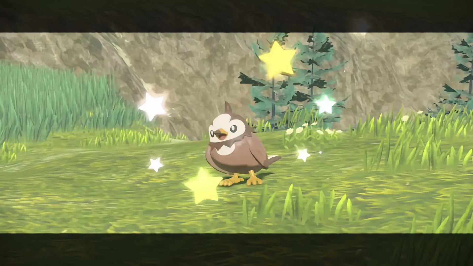
Shiny Pokémon are rare variants with unusual colours. When a Shiny Pokémon appears in the wild or from its Poké Ball, it is accompanied by a sound effect and a flash of light and stars.
28 Down
Solution
Clue
LOPE
Run from training under large officer (4)
The initialism PE (“training”, as in physical education) after (“under”, since this is a vertical clue) the letters L (short for “large”) and O (short for “officer”).
The surface clue refers to Zisu, the captain of the Galaxy Team Security Corps, who can be optionally battled at the training grounds.
Hidden message
Hidden message
Eagle-eyed solvers may notice the thematic message spelled out by the top and
bottom rows of the puzzle: ARCEUS LEGEND.
Shawn Mendes’ song “Lost in Japan” has had me geographically confused since I first heard it covered by Scary Pockets. If you haven’t listened to the lyrics, the song is about a person who is thinking about their crush and the possibility of taking a last-minute flight to Japan to see them.
The question I can’t get off my mind is: where is the song supposed to be taking place?
The chorus goes:
Do you got plans tonight?
I’m a couple hundred miles from Japan, and I
I was thinking I could fly to your hotel tonight
‘Cause I can’t get you off my mind
from which we can infer that
the crush is somewhere in Japan
the singer is outside of Japan, and
both people are close enough to an international airport for one to entertain the idea of flying to the other’s hotel.
The most likely candidates for airports within “a couple hundred miles from Japan” are in South Korea.
The area within 100 to 500 miles of a Japanese airport with year-round
scheduled international flights.
When I first considered the geography of the song, I was satisfied with that answer: couple of hundred miles, South Korea, that sounds about right. But then I noticed the opening lyrics:
All it’d take is one flight
We’d be in the same time zone
That would seem to rule out South Korea, which is in the same time zone as Japan. With the closest locations out of the picture, we have to stretch our interpretation of the song. Here are the possibilities I can see.
The singer could be in Shanghai
Shanghai is 500 miles (in different directions) from Okinawa and Kyūshū Islands. Shanghai Pudong International Airport was the eighth-busiest airport in the world when “Lost in Japan” was released, and has plenty of routes to both Naha and Nagasaki.
This is probably the most plausible answer if we make the thematically appropriate assumption that the lovestruck protagonist is downplaying the distance in order to convince themself that taking a last-minute flight is a good idea.
The singer could be in Vladivostok
Vladivostok is also within 500 miles of New Chitose Airport in Sapporo. This possibility is pretty funny, but unfortunately it’s ruled out by logistics. The only regular flight I could find between the two was only opened by Ural Airlines after “Lost in Japan” was released, and did not last long before world events shut it down permanently.
The singer could be in Taipei
There’s only one location that geographically fits the lyrics exactly: our protagonist is in Taiwan, and their crush is less than 200 miles away in Ishigaki on Japan’s southwesternmost inhabited archipelago.
With a creative enough interpretation, this is also consistent with the second verse:
Do I gotta convince you
That you shouldn’t fall asleep?
It’ll only be a couple hours
And I’m about to leave.
The singer is presumably in a hurry to leave because they have just checked the timetable for the only direct flight from Taipei to Ishigaki, which runs on Wednesdays and Saturdays during the tourist season. The flight is short enough that “a couple hours” is realistic if customs is quick.
The line about falling asleep is, of course, a request for the romantic interest to skip their usual afternoon nap, since China Airlines flight 124 arrives at 11:35am.
The time it takes to properly roast a whole turkey is proportional to its weight to the ⅔ power. My old mathematical modelling textbook specifically recommends 45 minutes per lb2/3 when cooked at 350℉.
For a spherical turkey of uniform thermal conductivity α and density ρ, a precise formula has been derived:
t=ln(Th−Tf2(Th−T0))π2α1(4πρ3)2/3m2/3
where the oven is set at Th and the center of the turkey needs to reach a temperature of Tf from T0.
The more general ⅔ power law does not depend on unrealistic assumptions about the turkey’s shape or thermodynamic properties; it can be derived from pure dimensional analysis and applied to turkey-shaped meat-based objects by fitting a curve to specific cook times used by chefs.
Since the ’50s, Alberta has engaged in a deliberate effort to prevent rats from entering the province. Fortunately, rats can’t survive in the wild in Alberta, so they have pest inspectors regularly check every premise within a 29 x 600 km control zone from Montana to Cold Lake. Pet rats are illegal.
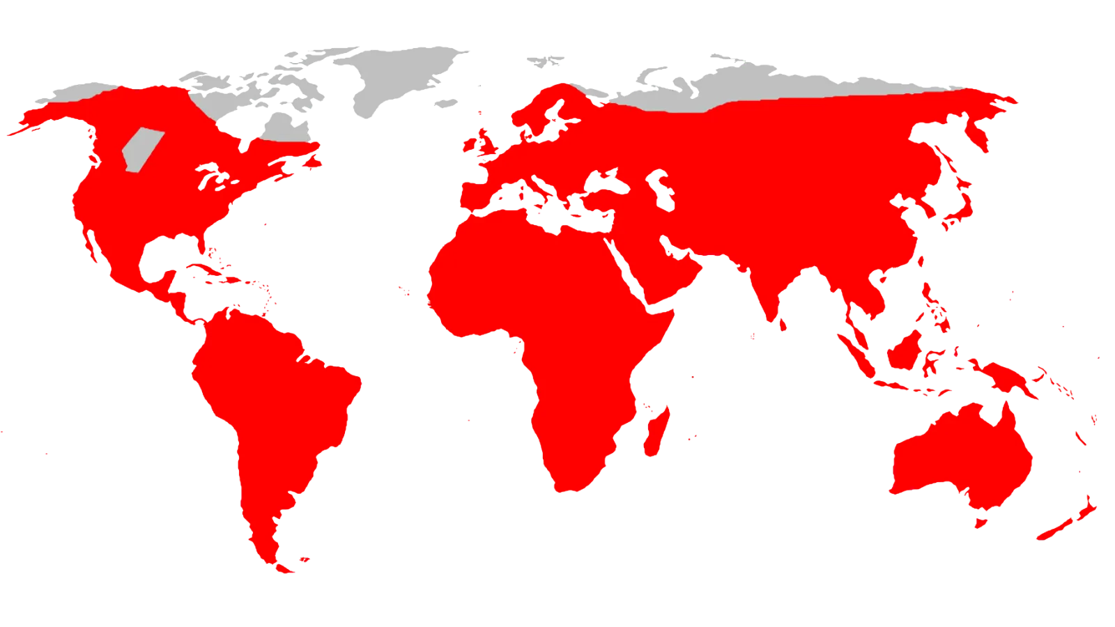
The rat-free status of Alberta led to a Wikipedia edit war over whether the province should appear on a map of the brown rat’s habitat. At some point it was decided to remove the map entirely from the English-language entry for Rattus norvegicus, but its presence on other Wikimedia projects means the edit war still rages on to this day.
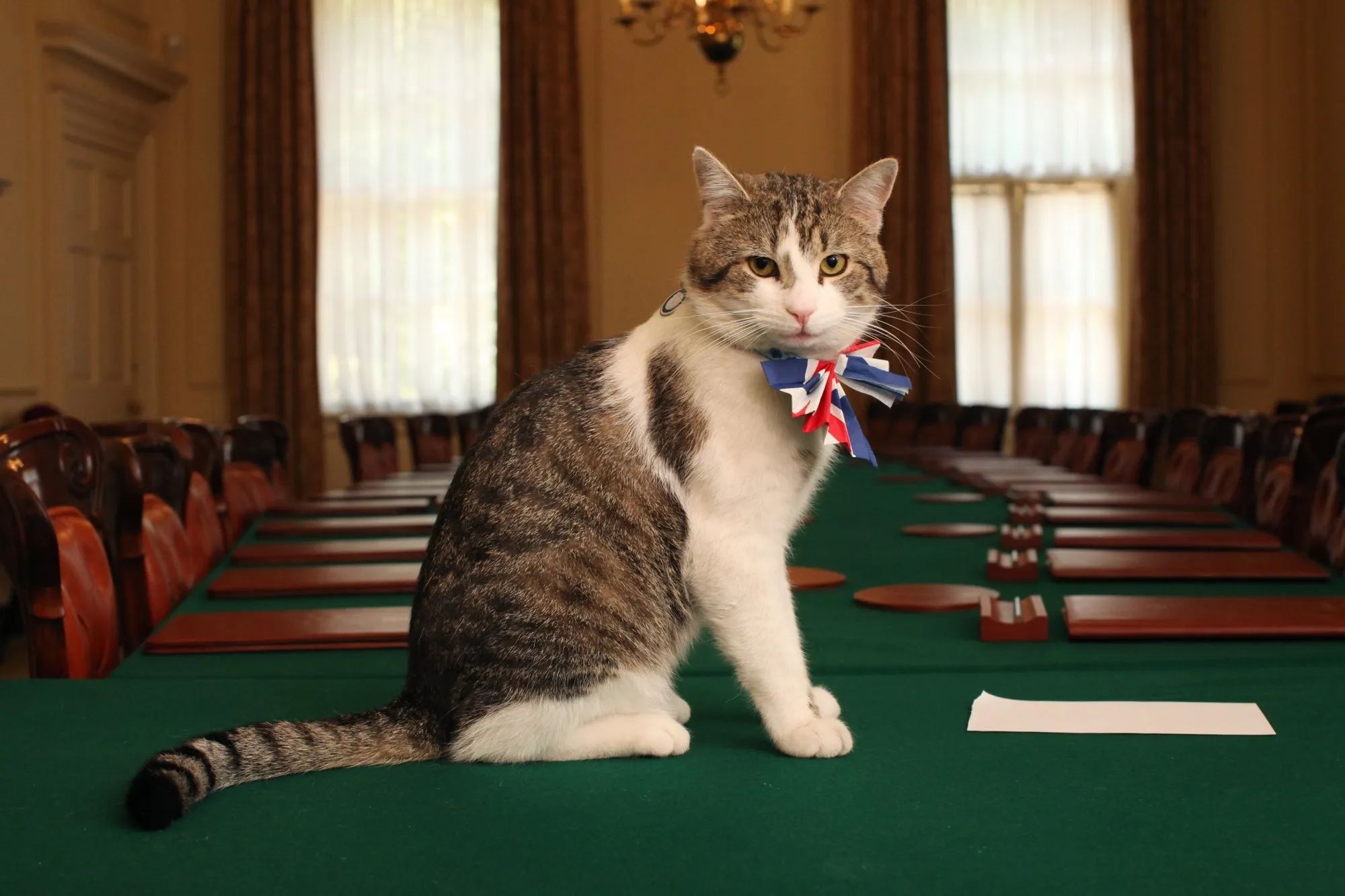
The official title of Chief Mouser to the Cabinet Office is held by a cat in charge of keeping mice under control at the UK Prime Minister’s office at 10 Downing Street. The current incumbent is Larry.
It was once commonplace to employ cats as mousers, so Larry is not unique; the UK Post Office employed a cat named Tibs the Great for many years and Canada’s Parliament had its own cat colony.
Vessel Finder is a map showing the current location of container ships, cruise ships, fishing boats, and other nautical vessels. It aggregates data from automatic identification systems which all sufficiently large boats are required to be fitted with.
The length distribution of tweets has shifted in response to raised character limits, but it’s still the case that a disproportionate number of tweets use all the characters they’re given.
A sample of tweets gathered in 2019 still exhibit a telltale spike approaching the character limit, but it is smaller than the tweet distribution from a decade earlier. The peak of the curve has also shifted leftwards, to 15 characters, due to a separate change in 2016 that excluded media attachments and certain at-mentions from the character count.
The most interesting feature of the above graph is unfortunately an artifact of the dataset — the massive spike at 105 characters can be blamed on a spambot network broadcasting identical copies of the same tweet when the dataset was collected.
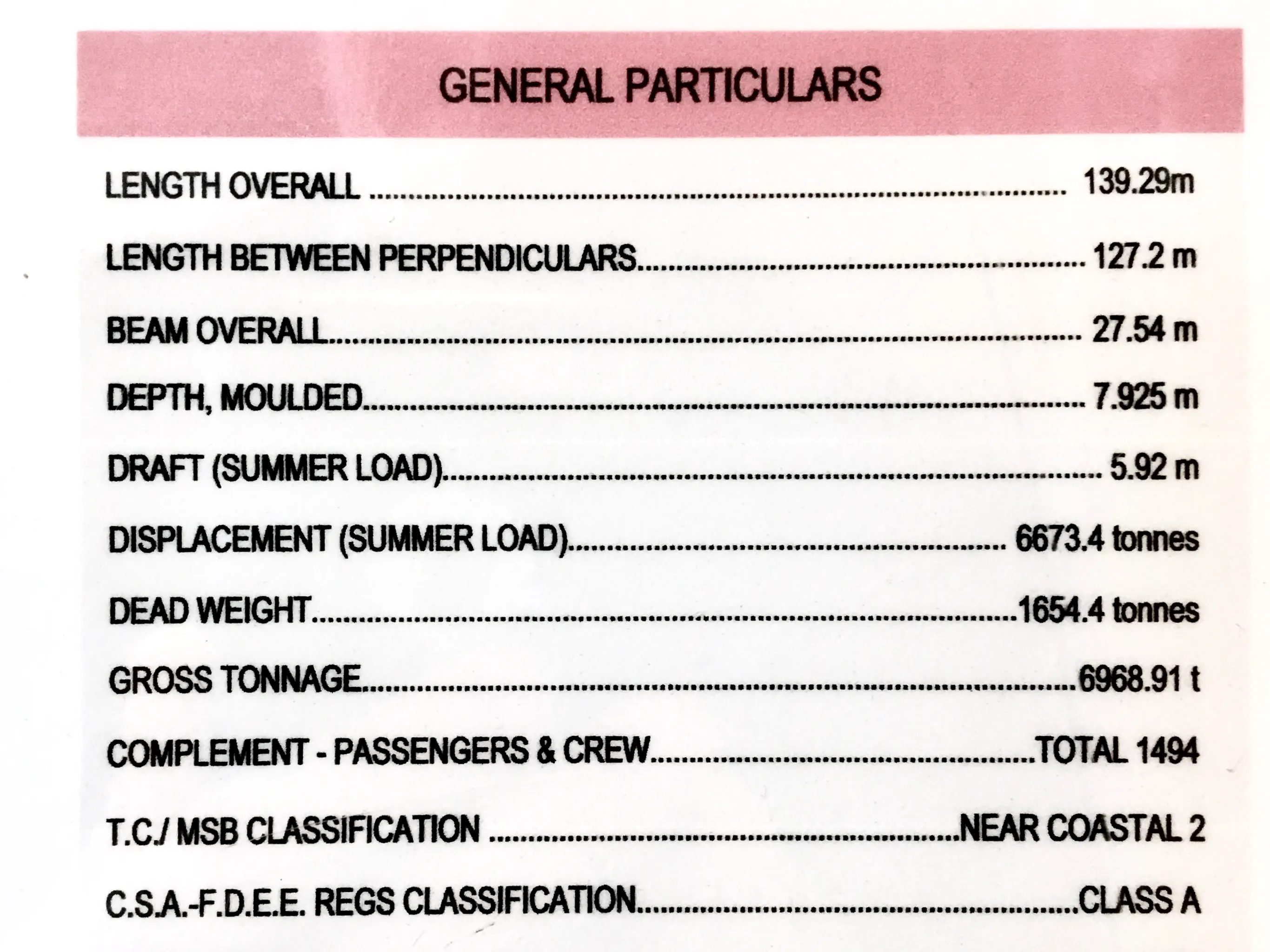
“General particulars” is an excellent phrase that deserves to catch on more widely than its current context of legally-mandated notices on boats.
(Boats are required by international law to have a wheelhouse poster listing their “general particulars”, i.e., a list of statistics, properties, and other bits of information necessary to get a basic view of the vessel.)
The head of a sunflower is actually hundreds of smaller flowers working together to attract pollinators. Each large yellow petal is its own individual flower, and the bits in the middle are tiny five-pointed flowers if you look closely.
Pokémon Gold and Silver’s roaming legendary beasts move randomly from route to route instead of sticking to a fixed habitat. By analyzing their behaviour using the math of random walks on graphs, I can finally answer a question that’s bugged me since childhood: what’s the best strategy to find a roaming Pokémon as quickly as possible?
Catching a roaming Pokémon is a graph pursuit game, but in practice the optimal strategy doesn’t involve a chase at all. Raikou and the other roaming Pokémon move every time the player crosses the boundary from one location to another, regardless of how long that takes. So if we repeatedly cross the boundary by taking one step forward and one step back, Raikou will effortlessly speed across the map.
The easiest strategy, then, is to choose a centrally-located location and hop back and forth until Raikou comes to us. The question is what location gives the best results.
Vertices of maximum degree
When left to its own devices, a random walk in a graph G returns to a vertex v every
deg(v)2∣E(G)∣
steps. This suggests that the best place to find Raikou is a vertex of maximum degree on the graph corresponding to the Johto map.
The routes of Johto coloured according to their corresponding vertex degrees.
This puts Johto Route 31 as the top candidate, since it’s the only route adjacent to five other routes (Routes 30, 32, 36, 45, and 46) on the roaming Pokémon’s trajectory.
Vertices with minimum average effective resistance
Of course, we don’t intend to leave Raikou to its own devices—we’re going to try to catch it whenever it’s on our route! If it gets away, it will flee to a random location that can be anywhere on the map, regardless of whether it is adjacent or not. This wrinkle means we’re not exactly trying to find the vertex with the fastest return time; we’re really trying to minimize
∣V(G)∣1u∈V(G)∑T(u,v),
where T(u,v) is the expected time for a random walk starting at u to first reach our vertex v.
How do we compute this value? According to Tetali, we replace all of the edges with 1-ohm resistors and measure the effective resistances Rxy between each pair of nodes x,y in the corresponding electrical network. Then
T(u,v)=21w∈V(G)∑deg(w)(Ruv+Rvw−Ruw).
It seems very appropriate to use the math of electrical networks to catch the electric-type Raikou! Unfortunately, there’s no references to effective resistance or Tetali’s formula in its Pokédex entry.
Effective resistance can be computed by hand using Kirchoff’s and Ohm’s Laws, but it’s much easier to plug it into SageMath, which uses a nifty formula based on the Laplacian matrix of the graph.1
Expected capture time when moving between a given route and an adjacent town
Route 31 comes out on top again by this measure: if Raikou starts from a random location, it will come to this route sooner on average than any other single location.
Vertex pairs with minimum average effective resistance
But this still isn’t the final answer. The above calculations assume we’re hopping between a route (where we can catch Raikou) and a town (where we can’t).1 What if we go to a boundary where either side gives us a chance for an encounter?
There are only four pairs of routes in Johto where this is possible. The expected capture time when straddling one of these special boundaries can be computed using the same kinds of calculations. All four route pairs yield an expected capture time faster than relying on any individual route — enough to dethrone Route 31!
Expected capture time when moving between adjacent locations. Each pair has
two expected capture times, shown in different shades, depending on which
route is considered the starting point.
Source code
Source code
G =Graph({29:[30,46],30:[31],31:[32,36,45,46],32:[33,36],33:[34],34:[35],35:[36],36:[37],37:[38,42],38:[39,42],42:[43,44],43:[44],44:[45],45:[46]})
def hitting*time(routes, u, v):H0= H(routes)R=lambdax,y: R_matrix(routes)[H0.vertices().index(x)][H0.vertices().index(y)]return1/2* sum(H0.degree(w)\_ (R(u,v) + R(v,w) - R(u,w)) for w in H0.vertices())
{(x, y): mean([ hitting_time((x,y),(u,0),(x,0))for u in G.vertices()])for(x, y)in[(30,31),(31,30),(35,36),(36,35),(36,37),(37,36),(45,46),(46,45)]}
Although Raikou will on average arrive at Route 31 faster than any other route, the best place to catch the roaming legendary Pokémon is the boundary between Johto Routes 36 and 37. Hop back and forth between those two routes, and before you know it, you’ll be one step closer to completing your Pokédex!
Specifically, the calculations were done on the tensor
product of K2 and
the graph representing Raikou’s possible moves between the Johto routes.
Not all 26 letters of the alphabet appear on BC license plates. Six are missing — and the reason goes all the way back to 1970, when BC switched from issuing sequential plate numbers to an alphanumeric system.
One [story] is that the stamps used by employees of the MVB for compiling licensing documents in 1960s only had enough space for ten (10) characters.
The other is that when the province upgraded the machinery at the Oakalla Plate Shop in the mid-1950s, it was designed to accommodate a maximum row of ten (10) different dies for each of the six columns that might be used in the license plate’s serial.
Regardless of which, if any of these stories is the correct one, the alphabet was broken into two blocks of ten letters with the first block comprising A, B, C, D, E, F, G, H, J, and K with “I” excluded as it too closely resembled the number one.
The second block of letters used on BC passenger license plates was L, M, N, P, R, S, T, V, W, and X. The letters I and O were obviously too similar to 1 and 0, and Q was apparently also skipped due to its resemblance to zero.1 I imagine U was excluded instead of X to minimize the number of unusable plate numbers containing rude words. Y and Z missed out just because they’re at the end of the alphabet.
BC has issued several different plate series since the ’70s and the manufacturing process has presumably changed since then, but I believe the letters have remained the same. To this day, I have still never seen an I, O, Q, U, Y, or Z on a BC passenger car.
Keep an eye out for other types of vehicles, though. Motorcycle plates starting with U, Y, and Z were issued in 2012–14, 2017–18, and 2019–20 respectively, and the letters can also be spotted on plates assigned to commercial trucks.
I recall asking this at the end of my driver’s test many years ago, and being
given this answer by an ICBC employee. This is supported by the fact that
other kinds of plates are issued with U, Y, and Z but not the three ambiguous
characters. That said, I’m a little curious why S was not also skipped due to
its resemblance to the number 5.


