Numbers like $\pi$ and $\sqrt{2}$ are irrational. Are they called that because they are unreasonable? Or is it just because they just can’t be expressed as a ratio of two integers?

As it turns out, this question is even harder to answer in Ancient Greek. On the one hand, the word used by (e.g.) Euclid to describe irrational lengths (ἄλογος) comes from adding the negative prefix ἄ- to the word for ratio (λόγος). On the other hand, λόγος and ἄλογος had a lot of other meanings.

Ἄλογος could mean unexpected, which would be an appropriate description of the newly-discovered irrational numbers. Or it could mean unspeakable — in the literal sense, although the figurative sense fits with the (possibly fictitious) cover-up by the Pythagoreans. The word could also mean speechless or incapable of reasoning.

It’s fascinating to see how translators (and later mathematicians) decided to resolve the polysemy of ἄλογος:

• Latin translations of Greek works used ratio for λόγος and irrationalis for ἄλογος. These were actually imported into mathematical English before their non-technical meanings.
• Early Arabic mathematicians called $\sqrt{2}$ a deaf root (جذر أصم) in reference to the “speechless” meaning of ἄλογος. This got translated back to Latin as surd, a now-archaic term for (irreducible) roots.
• In modern Arabic, the phrase is “non-fractional number” (عدد غير كسري).
• In modern Greek, irrational numbers are now called inexpressible (άρρητος).

The Pythagorean theorem states that, for a right triangles with side lengths $a, b$ and hypotenuse $c$:

There are many proofs, but my favourite for its geometric simplicity is the following proof by rearrangement.

In case you ever have need for a large-ish prime number, here are a few that are easy to remember:

• 314159 ($\lfloor \pi \cdot 10^5 \rfloor$)
• 8675309 (Jenny’s number)
• 1000000007 (a billion and seven)
• 2147483647 ($2^{31}-1$, i.e. INT_MAX)
• 11111111111111111111111 (twenty-three ones)
• 1000000000000066600000000000001 (Belphegor’s prime)

A while ago I arbitrarily decided that I needed a favourite three-digit number (don’t ask) and ended up choosing 216. It’s a nice cube number — 6×6×6 — and can also be expressed as a sum of three smaller cubes:

The Wikipedia article for the number has a diagram showing one way to reassemble a 6×6×6 cube into three smaller cubes, but I’ve been playing around looking for other, more aesthetically pleasing methods. Here’s one I found.

First, we break the 6×6×6 cube into its 4×4×4 interior, six 4×4×1 faces, twelve 4×1×1 edges, and eight 1×1×1 corners:¹ i.e.,

The 4×4×1 faces can be combined with seven of the edges and one of the corners to build a 5×5×5 cube. The remaining five edges can be split into ten 2×1×1 chunks and arranged with the remaining seven corners to form a 3×3×3 cube.

There are many more ways to construct three cubes from the pieces of a 6×6×6 cube. What’s your favourite?

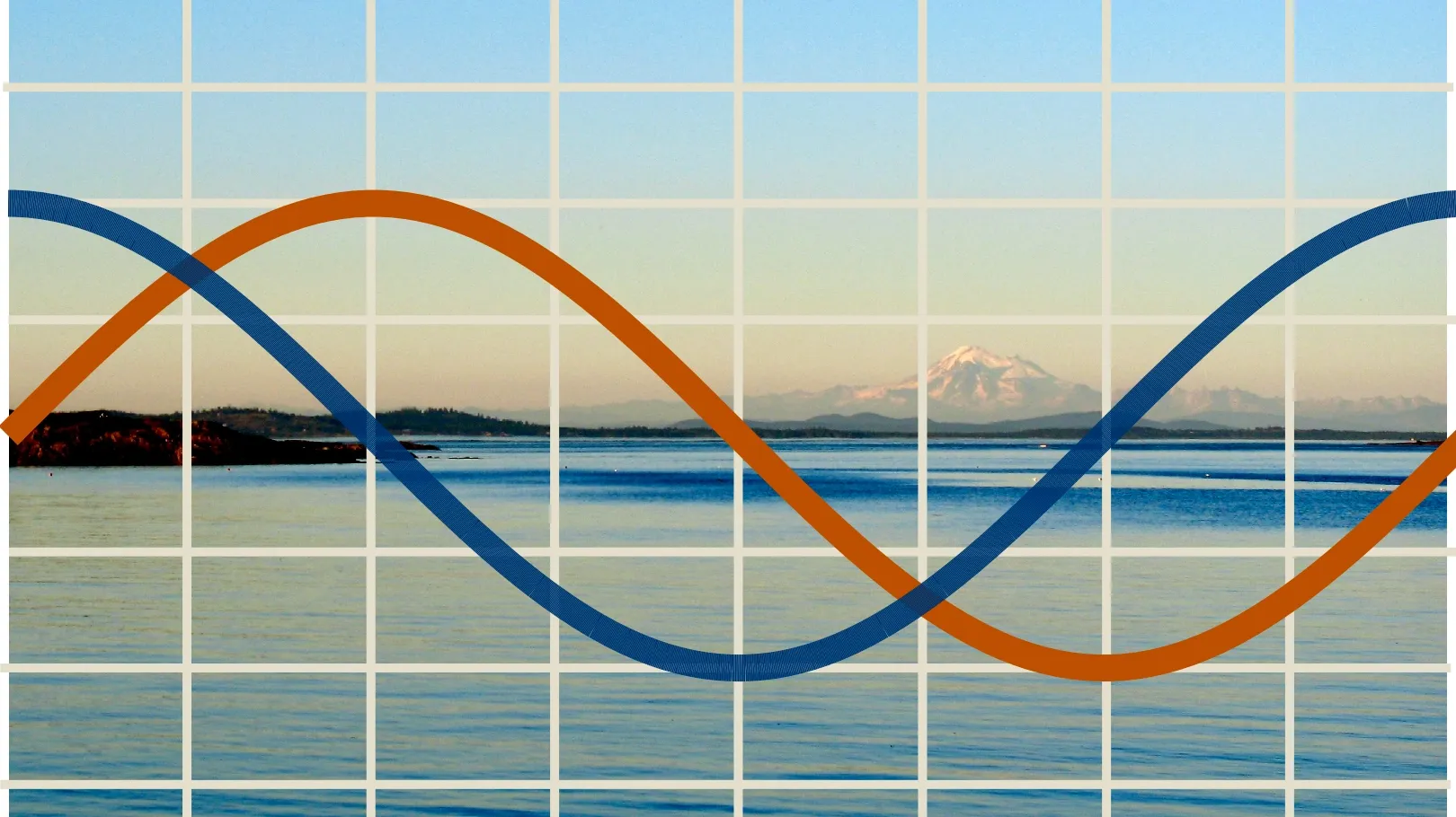
You can get a really good approximation of a sinusoidal curve from twelve equally-spaced line segments of slope 1/12, 2/12, 3/12, 3/12, 2/12, 1/12, -1/12, -2/12, -3/12, -3/12, -2/12, and -1/12, respectively.

This approximation, known as the rule of twelfths, rounds $\sqrt{3} \approx 5/3$ but otherwise uses exact values along the curve.

I learned about the rule of twelfths from a kayaking instructor and guide, who used it to estimate the tides. In locations and seasons with a semidiurnal tide pattern, the period of the tide is roughly 12 hours, and the rule of twelfths tells you what the water will be doing in each hour.

For example, if you know that the difference between low and high tide is 3 feet, then you can quickly estimate that it the tide will rise by about 3 inches in the first hour, 6 inches in the second, 9 inches in the third and fourth, 6 inches in the fifth hour, and 3 inches in the last hour before high tide.

The time it takes to properly roast a whole turkey is proportional to its weight to the ⅔ power. My old mathematical modelling textbook specifically recommends 45 minutes per lb^2/3 when cooked at 350℉.

For a spherical turkey of uniform thermal conductivity $\alpha$ and density $\rho$, a precise formula has been derived:

where the oven is set at $T_h$ and the center of the turkey needs to reach a temperature of $T_f$ from $T_0$.

The more general ⅔ power law does not depend on unrealistic assumptions about the turkey’s shape or thermodynamic properties; it can be derived from pure dimensional analysis and applied to turkey-shaped meat-based objects by fitting a curve to specific cook times used by chefs.

Pokémon Gold and Silver’s roaming legendary beasts move randomly from route to route instead of sticking to a fixed habitat. By analyzing their behaviour using the math of random walks on graphs, I can finally answer a question that’s bugged me since childhood: what’s the best strategy to find a roaming Pokémon as quickly as possible?

Catching a roaming Pokémon is a graph pursuit game, but in practice the optimal strategy doesn’t involve a chase at all. Raikou and the other roaming Pokémon move every time the player crosses the boundary from one location to another, regardless of how long that takes. So if we repeatedly cross the boundary by taking one step forward and one step back, Raikou will effortlessly speed across the map.

The easiest strategy, then, is to choose a centrally-located location and hop back and forth until Raikou comes to us. The question is what location gives the best results.

Vertices of maximum degree

When left to its own devices, a random walk in a graph G returns to a vertex v every

steps. This suggests that the best place to find Raikou is a vertex of maximum degree on the graph corresponding to the Johto map.

This puts Johto Route 31 as the top candidate, since it’s the only route adjacent to five other routes (Routes 30, 32, 36, 45, and 46) on the roaming Pokémon’s trajectory.

Vertices with minimum average effective resistance

Of course, we don’t intend to leave Raikou to its own devices—we’re going to try to catch it whenever it’s on our route! If it gets away, it will flee to a random location that can be anywhere on the map, regardless of whether it is adjacent or not. This wrinkle means we’re not exactly trying to find the vertex with the fastest return time; we’re really trying to minimize

where $T(u, v)$ is the expected time for a random walk starting at $u$ to first reach our vertex $v$.

How do we compute this value? According to Tetali, we replace all of the edges with 1-ohm resistors and measure the effective resistances $R_{xy}$ between each pair of nodes $x, y$ in the corresponding electrical network. Then

It seems very appropriate to use the math of electrical networks to catch the electric-type Raikou! Unfortunately, there’s no references to effective resistance or Tetali’s formula in its Pokédex entry.

Effective resistance can be computed by hand using Kirchoff’s and Ohm’s Laws, but it’s much easier to plug it into SageMath, which uses a nifty formula based on the Laplacian matrix of the graph.¹

Route 31 comes out on top again by this measure: if Raikou starts from a random location, it will come to this route sooner on average than any other single location.

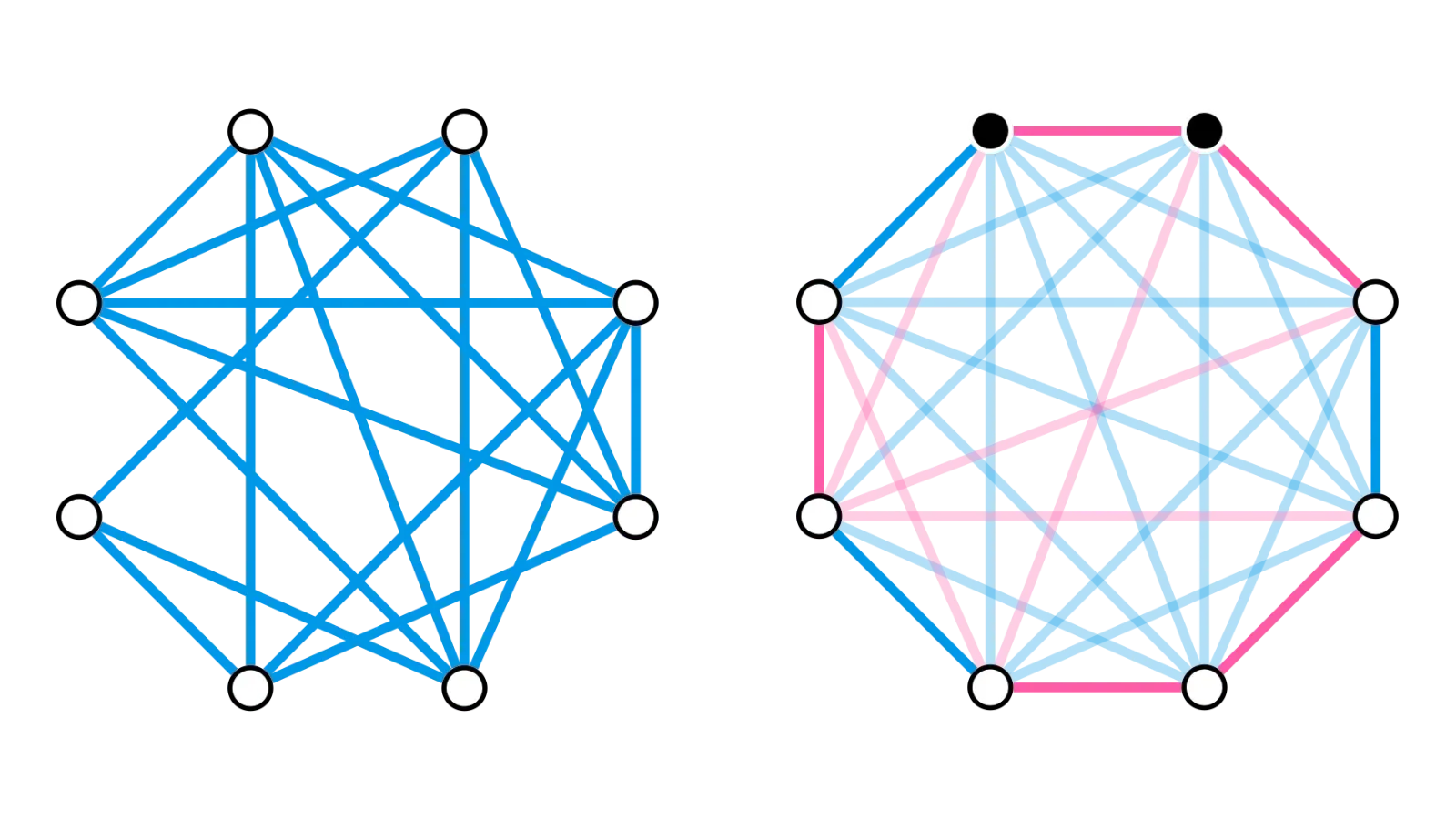
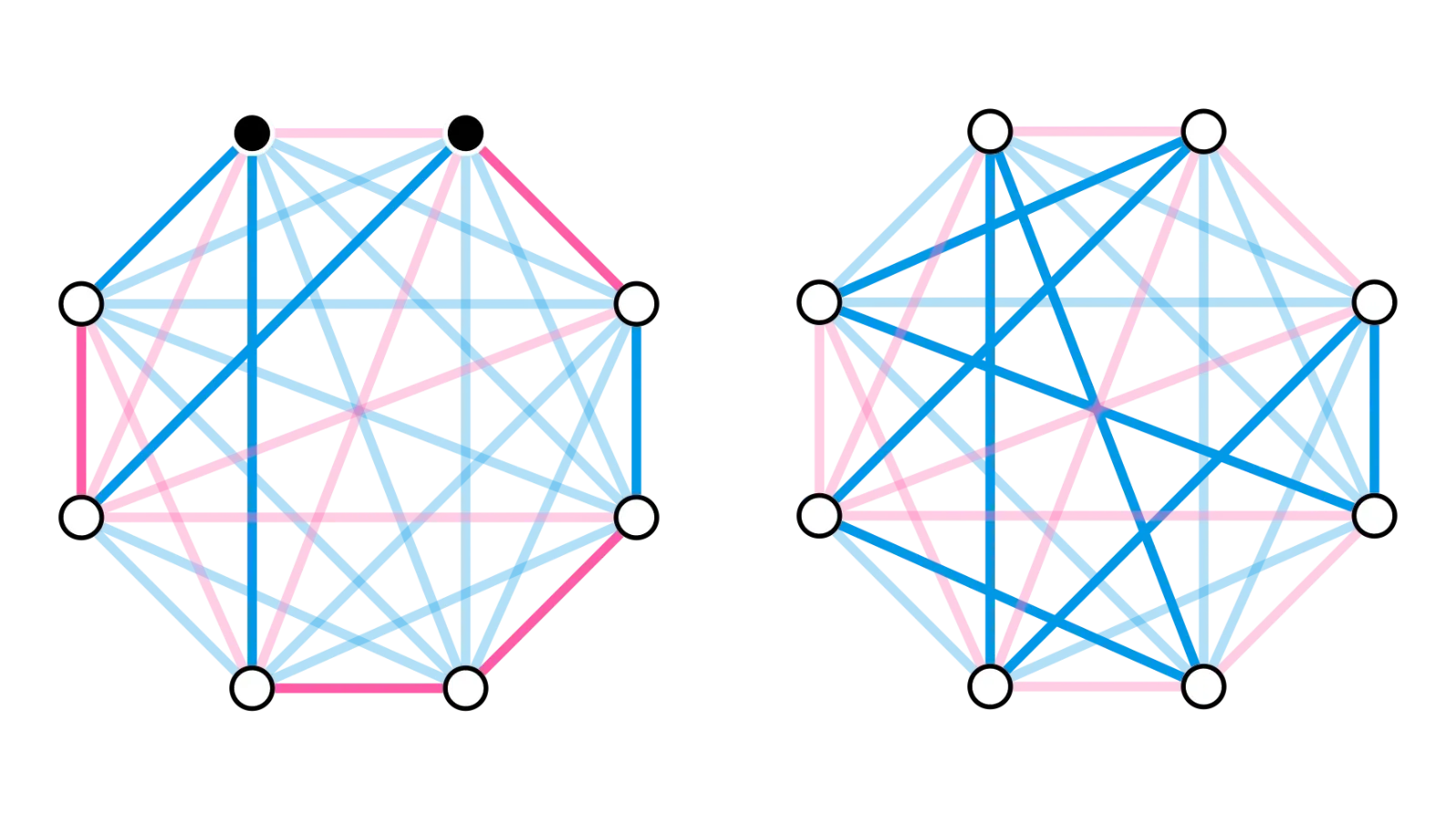
Vertex pairs with minimum average effective resistance

But this still isn’t the final answer. The above calculations assume we’re hopping between a route (where we can catch Raikou) and a town (where we can’t).1 What if we go to a boundary where either side gives us a chance for an encounter?

There are only four pairs of routes in Johto where this is possible. The expected capture time when straddling one of these special boundaries can be computed using the same kinds of calculations. All four route pairs yield an expected capture time faster than relying on any individual route — enough to dethrone Route 31!

Source code

G = Graph({ 29: [30, 46], 30: [31], 31: [32, 36, 45, 46], 32: [33, 36], 33: [34], 34: [35], 35: [36], 36: [37], 37: [38, 42], 38: [39, 42], 42: [43, 44], 43: [44], 44: [45], 45: [46] })

R_matrix = G.effective_resistance_matrix()

def R(u, v): return R_matrix[G.vertices().index(u)][G.vertices().index(v)]

def hitting*time(u, v): return 1/2 * sum(G.degree(w) \_ (R(u,v) + R(v,w) - R(u,w)) for w in G.vertices())

def avg_hitting_time(v): return mean([hitting_time(u, v) for u in G.vertices()])

{ v: avg_hitting_time(v) for v in G.vertices() }

# account for parity

H = G.tensor_product(graphs.CompleteGraph(2)) R_matrix = H.effective_resistance_matrix()

def R(u, v): return R_matrix[H.vertices().index(u)][H.vertices().index(v)]

def hitting*time(u, v): return 1/2 * sum(H.degree(w) \_ (R(u,v) + R(v,w) - R(u,w)) for w in H.vertices())

def avg_hitting_time(v): return mean([hitting_time((u,0),(v,0)) for u in G.vertices()])

{ v: avg_hitting_time(v) for v in G.vertices() }

# Final

@CachedFunction def H(routes=None): if routes is None: return G.tensor_product(graphs.CompleteGraph(2)) else: x, y = routes graph = H(None).copy() graph.merge_vertices([(x, 0), (y, 1)]) return graph

@CachedFunction def R_matrix(routes): return H(routes).effective_resistance_matrix()

def hitting*time(routes, u, v): H0 = H(routes) R = lambda x,y: R_matrix(routes)[H0.vertices().index(x)][H0.vertices().index(y)] return 1/2 * sum(H0.degree(w) \_ (R(u,v) + R(v,w) - R(u,w)) for w in H0.vertices())

{ (x, y): mean([ hitting_time((x,y), (u,0), (x,0)) for u in G.vertices() ]) for (x, y) in [(30,31), (31,30), (35,36), (36,35), (36,37), (37,36), (45,46), (46,45)] }

Although Raikou will on average arrive at Route 31 faster than any other route, the best place to catch the roaming legendary Pokémon is the boundary between Johto Routes 36 and 37. Hop back and forth between those two routes, and before you know it, you’ll be one step closer to completing your Pokédex!

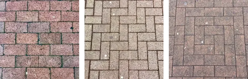
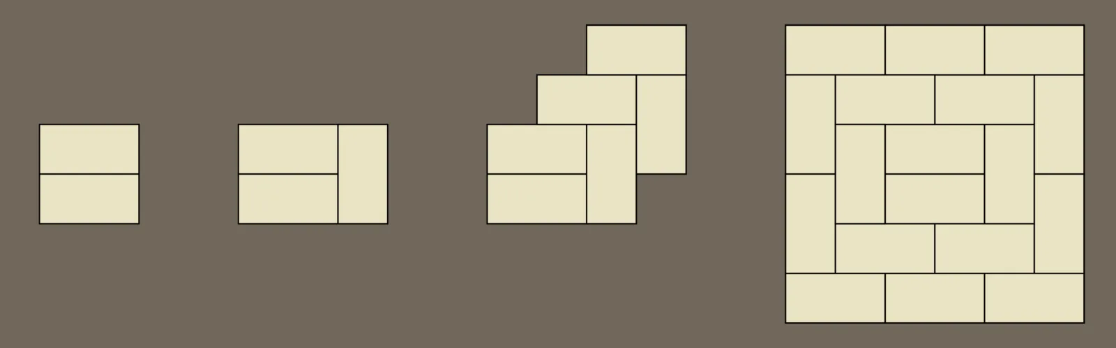
Brick pavements and tatami mats are traditionally laid out so that no four meet at a single point to form a ┼ shape. Only a few ┼-free patterns can be made using $1\times 1$ and $1\times 2$ tiles, but the addition of $2\times 2$ tiles provides a lot more creative flexibility.

When I discussed tatami tilings with my relative Oliver Linton, he suggested applying similar rules to other brick sizes to make beautiful tiling patterns. The tatami condition alone does not provide enough of a constraint to mathematically analyze tilings with arbitrary shapes and sizes, but it is a good starting point when looking for interesting patterns.

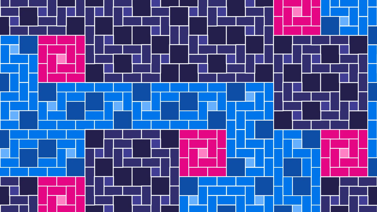
With the addition of $2\times 2$ square tiles, it’s possible to construct rectangular blocks that fit together to tesselate the plane while preserving the four-corner rule.

This opens the door to self-similar tilings, which I’m very interested in! The goal is to use $1 \times 1$, $1 \times 2$, and $2 \times 2$ tiles to construct $n\times n$, $n \times 2n$, and $2n \times 2n$ blocks which can be put together in the exact same way to make increasingly intricate $n^k \times n^k$ tilings that maintain the tatami condition.

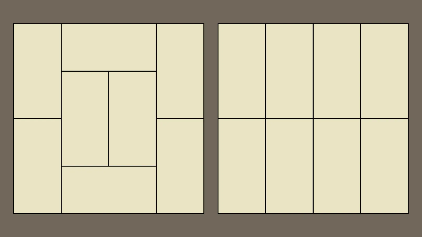
The simplest non-trivial example I could find involves a set of $5\times 5$, $10 \times 10$, and two $5\times 10$ rectangular tilings.

Starting with any of these four layouts, we can replace each of the $1\times 1$, $2\times 2$, and $1\times 2$ bricks with a corresponding $5\times 5$, $10\times 10$, or $5\times 10$ rectangular tiling in the correct orientation. (This will produce a few four-corner intersections, but we can fix these by merging adjacent pairs of $1\times 2$ bricks.)

Repeatedly performing this operation gives an infinite sequence of tilings, but can we say they converge to anything? A tiling $T$ can be identified with its outline $\partial T$ (i.e. the set of points on boundaries between two or more tiles). Note that if a point is in $\partial T_i$, then it will be in every subsequent $\partial T_j$ unless it is one of the few bricks merged in $\partial T_{i+1}$. So we might sensibly define the limiting object of the tiling sequence $T_i$ as the union

This self-similar dense path-connected set satisfies the topological equivalent of the “four corners rule” — a pretty interesting list of mathematical properties!

The same strategy could be applied to other sets of $(2n+1)\times (2n+1)$, $(4n+2)\times (4n+2)$, and $(2n+1)\times (4n+2)$ tiles with similar boundaries. What’s the prettiest brickwork fractal you can find?

Although I’ve left academia, Bojan Mohar and I have published a new paper in the proceedings of SODA exploring the “perimeter” measure that plays a key role in my doctoral research. It is mostly based on Chapter 4 of my PhD thesis.

I have succesfully defended my PhD thesis! It’s “packed” with results on graph immersions with parity restrictions, and “covers” odd edge-connectivity, totally odd clique immersions, and a new submodular measure that’s intimately connected with both.

I am grateful to NSERC for funding my degree with a Alexander Graham Bell Canada Graduate Scholarship, and to my supervisor Bojan Mohar.

I have a new paper, coauthored with my supervisor Bojan Mohar and colleague Hehui Wu and presented at the SIAM Symposium on Discrete Algorithms! It is my first foray into graph immersions with parity restrictions.

I am grateful to NSERC for supporting this research through an Alexander Graham Bell Canada Graduate Scholarship.

I have a new paper published in Graphs and Combinatorics! It’s my favourite paper to come out of my research with Jing Huang at the University of Victoria — the third written chronologically, and the last to be published. The main result is that the structure of monopolar partitions in claw-free graphs can be fully understood by looking at small subgraphs and following their direct implications on vertex pairs.

One of the most recognizable features of Japanese architecture is the matted flooring. The individual mats, called tatami, are made from rice straw and have a standard size and $1 \times 2$ rectangular shape. Tatami flooring has been widespread in Japan since the 17th and 18th centuries, but it took three hundred years before mathematicians got their hands on it.

According to the traditional rules for arranging tatami, grid patterns called bushūgishiki (不祝儀敷き) are used only for funerals.¹ In all other situations, tatami mats are arranged in shūgishiki (祝儀敷き), where no four mats meet at the same point. In other words, the junctions between mats are allowed to form ┬, ┤, ┴, and ├ shapes but not ┼ shapes.

Shūgishiki tatami arrangements were first considered as combinatorial objects by Kotani in 2001 and gained some attention after Knuth including them in The Art of Computer Programming.

Construction

Once you lay down the first couple tatami, you’ll find there aren’t many ways to extend them to a shūgishiki. For example, two side-by-side tatami force the position of all of the surrounding mats until you hit a wall.

This observation can be used to decompose rectangular shūgishiki into

• $(m-2)\times m$ blocks forced by vertical tatami,
• $m \times m$ blocks forced by horizontal tatami, and
• $1\times m$ strips of vertical tiles,

and to derive their generating function

Four-and-a-half tatami rooms can also be found in Japanese homes and tea houses, so naturally mathematicians have also looked into tatami tilings with half-tatami. Alejandro Erickson’s PhD thesis reviews and extends the research into this area. Alejandro has also published a book of puzzles about tatami layouts.

I have a new paper with Jing Huang in Graphs and Combinatorics! This was the culmination of my undergraduate research, and shows that a single strategy can be used to solve the monopolar partition problem in all graph classes for which the problem was previously known to be tractable, including line graphs and claw-free graphs.

This research was completed in the summer of 2010, my last undergraduate research term. I am grateful to NSERC for funding my work with a Undergraduate Student Research Award, and to my supervisor and coauthor Jing Huang.

I have successfully defended my master’s thesis on graph-transverse matching problems! It considers the computational complexity of deciding whether a given graph admits a matching which covers every copy of a fixed tree or cycle.

The thesis is related to my previous work on cycle-transverse matchings and $P_4$-transverse matchings and, roughly speaking, shows that H-transverse matchings are NP-hard to find when $H$ is a big cycle or tree, and tractable when $H$ is a triangle or a small tree.

I am grateful to NSERC for funding my degree with a Alexander Graham Bell Canada Graduate Scholarship, and to my supervisor Jing Huang.

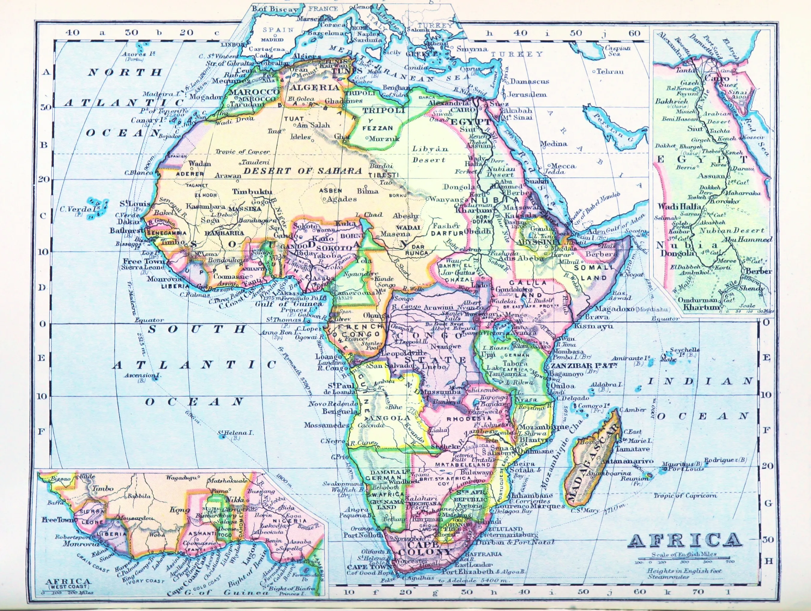
In 1852, then-student Francis Guthrie wondered any if possible map required more than four colours. By the end of the century, Guthrie and his fellow colonists had drawn a map on Africa that needed five.

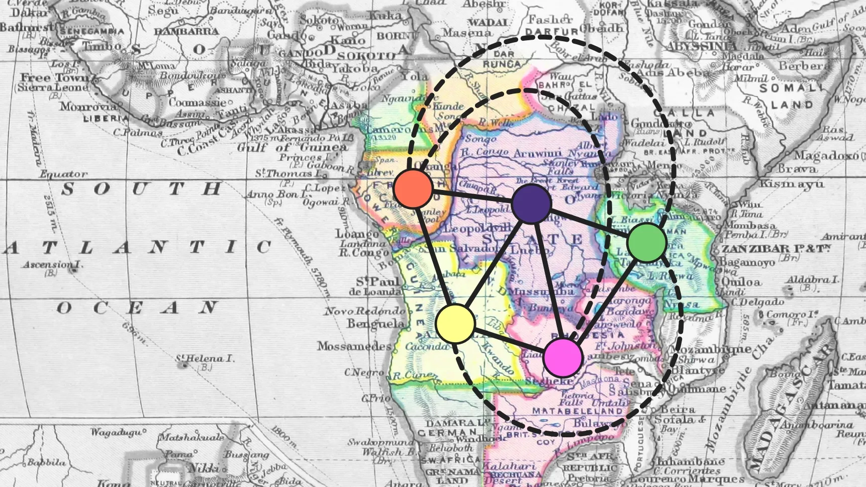
The Four-Colour Theorem says that, no matter what the borders on your map are, you only need four colours to make sure that neighbouring regions are coloured differently. The theorem doesn’t apply if you let some regions claim other disconnected regions as their own, and in fact the map of European claims on Africa required five colours by the end of the 19th century.

Francis Guthrie, who moved to the South African Cape Colony in 1861, could well have owned a map like the above. Five colours are necessary to properly colour the land that Britain (red), France (orange), Portugal (yellow), Germany (green), and Belgium’s King Leopold II (purple) decided should belong to them.

Five territorities in the center are key to the map colouring:

The boundaries between these colonies separate seven different pairs of empires. Borders between other African colonies account for the other three possible sets of neighbours:

• French Congo was next to German Kamerun;
• German East Africa to Portuguese Mozambique; and
• French claims in the Ubangi-Chari area were next to Anglo-Egyption Sudan.

In short, the adjacency graph between these empires was the complete graph $K_5$.

Pokémon Gold and Silver introduced the roaming legendary beasts: three one-of-a-kind Pokémon that move from route to route instead of sticking to a fixed habitat. Catching a roaming Pokémon amounts to winning a graph pursuit game — so what can we learn about it from the latest mathematical results?

To review the Pokémon mechanics, each species can normally be found in a handful of fixed habitats. If you want to catch Abra, you go to Route 24; if you’re looking for Jigglypuff, head to Route 46.

The legendary Entei, Raikou, and Suicune¹ are different. There’s only one of each species, each situated on a random route. Each time the player character moves to a new location, the roaming Pokémon each move to a randomly-selected route adjacent to the one they were just on. In graph theory terms, the player and Pokémon are engaged in a pursuit game where the Pokémon’s strategy follows a random walk.

The study of graph pursuit games is a fascinating and active area of research. Classically, researchers have asked how many “cops” it takes to guarantee the capture of an evasive “robber” travelling around a graph. Depending on the graph, many cops might be needed to catch a clever robber; there is a deep open problem about the worst-case cop numbers of large graphs.

Because the graph corresponding to the Pokémon region of Johto contains a long cycle as an isometric subgraph, its cop number is more than one — in other words, it’s possible that a roaming Pokémon could theoretically evade a lone Pokémon trainer forever! Fortunately, the legendary beasts play randomly, not perfectly, so the worst-case scenario doesn’t apply.

A random walk in an arbitrary $n$-vertex, $m$-edge graph can be expected to spend $\deg(v)/(2m)$ of its time at each location $v$, and to visit the whole graph after at most roughly $4n^3/27$ steps. So any trainer who isn’t actively trying to avoid Entei should end up bumping into it eventually — and an intelligent trainer should be able to do much better.

The first place to start is the “greedy” strategy I originally tried as a kid: every time Entei moves, check the map, and move to any route that gets me closer to them. After Entei makes its random move, the distance between us could be unchanged (with Entei’s move offsetting mine), or it could go down by one, or it could go down by two in the lucky $1/\Delta$ chance that Entei moves towards me. If I start at a distance of $\ell$ steps away from Entei and get lucky $\ell/2$ times, I’ll have caught up — so using a negative binomial distribution bound,

In the grand scheme of things, this isn’t too bad — especially if $\Delta$ is low. But it still takes a frustratingly large time for a 12-year-old, and in general it’s possible to do better.

Recently, Peter Winkler and Natasha Komarov found a strategy for general graphs which gives a better bound on the expected capture time. Somewhat counterintuitively, it involves aiming for where the robber was — rather than their current location — until the cop is very close to catching him. The Komarov-Winkler strategy has an expected capture time of $n+o(n)$, where $n$ is the number of locations on the map. This is essentially best possible on certain graphs, and is better than the above $\Delta\ell/2$ bound when the graph has vertices with large degree.

For graphs without high-degree vertices — like the Pokémon world map — it is possible that a simpler solution could beat the Komarov–Winkler strategy. The problem is: simpler strategies may not be simpler to analyse. In her PhD thesis, Natasha wondered whether a greedy algorithm with random tiebreakers could guarantee $n+o(n)$ expected capture time. It is an open question to find a general bound for the “randomly greedy” strategy’s expected performance that would prove her right.

Shortly after solving the monopolar partition problem for line graphs, Jing Huang and I realized that our solution could be used to solve the “precoloured” version of the problem, and then further extended to claw-free graphs. Jing presented our result at the French Combinatorial Conference and the proceedings have now been published in Discrete Mathematics.

I’ve published a new paper in the SIAM Journal on Discrete Mathematics! The work is the result of the research term I took as an undergraduate in the summer of 2009. It studies the edge versions of the monopolar and polar partition problems, and presents a linear-time solution to both.

I am grateful to NSERC for funding my work with a Undergraduate Student Research Award, and to my supervisor and coauthor Jing Huang.

Earlier this year, I presented the first results of what would become my master’s thesis at the International Workshop on Combinatorial Algorithms. The paper, coauthored with Jing Huang and Xuding Zhu, has now been published in the LNCS proceedings. It studies the computational complexity of the following problem: in a given graph, is there a matching which breaks all cycles of a given length?

I am grateful to NSERC for funding this research with a Alexander Graham Bell Canada Graduate Scholarship.

My most recent talk in UVic’s discrete math seminar presented three poetic proofs by Adrian Bondy… and three actual poems summarizing the ideas in each one.

Ore’s Theorem

A red-blue $K_n$:
bluest Hamilton circuit
lies fully in $G$.

Ore’s theorem states:

Let $G$ be a simple graph on $n \geq 3$ vertices such that $d(u) + d(v) \geq n$ for any nonadjacent $u, v$. Then $G$ contains a Hamilton cycle.

Bondy’s proof is roughly as follows. Colour the edges of $G$ blue and add red edges to make a complete graph. The complete graph on $n \geq 3$ vertices has no shortage of Hamilton cycles, so choose one and label it $v_1 v_2 \ldots v_n v_1$.

Consider the blue neighbours of $v_1$ on the cycle, and then move one vertex to the right along the cycle so you’re looking at the set

There are $d_G(v_1)$ of these vertices, and if $v_1 v_2$ is red (i.e. $v_1$ and $v_2$ are nonadjacent in $G$), then the theorem’s hypothesis tells us that

Since $v_2$ has only $n-1-d_G(v_2)$ red neighbours and is not itself in $S$, that means at least one vertex $v_{i+1} \in S$ is a blue neighbour of $v_2$. We can now replace $v_1 v_2$ and $v_i v_{i+1}$ in the cycle with the two blue edges $v_1 v_2$ and $v_2 v_{i+1}$ to get a Hamilton cycle of $K_n$ with at least one more blue edge than we had before.

We can make the same argument again and again until we have a Hamilton cycle of $K_n$ with no red edges. The cycle being blue means it lies entirely in $G$, which proves the theorem.

Brooks’ Theorem

Greedily colour,
ensuring neighbours follow
all except the last.

Choose the last vertex wisely:
friend of few or of leaders.

Brooks’ Theorem says:

If $G$ is connected and is not an odd cycle or a clique, then $\chi(G) \leq \Delta(G)$.

If $G$ is not regular, Bondy colours it as follows. Let $r$ be a vertex of smaller-than-maximum degree. If we consider the vertices in the reverse order of a depth-first search rooted at $r$, each vertex other than $r$ has at least one neighbour later in the order and at most $d(v)-1$ neighbours earlier. Greedily colouring in this order will assign one of the first $d(v) \leq \Delta(v)$ colours to each $v \neq r$, and at least one colour remains available for $r$ since its degree is strictly smaller than $\Delta(G)$.

If $G$ is regular, there are a few cases. If it has a cut vertex, we can break the graph into two (non-regular) parts, colour each of them separately, and put them back together. If it has a depth-first tree that branches at some point, then Bondy constructs an ordering similar to the one for the non-regular case: if $x$ has distinct children $y, z$ in the tree, $G$ can be ordered so $y$ and $z$ come first, $x$ comes last, and every other vertex has at least one neighbour later on in the order. A greedy colouring according to this order uses at most $\Delta(G)$ colours.

Finally, if $G$ is regular, 2-connected, and all of its depth-first trees are paths, it turns out that $G$ must be a chordless cycle, a clique, or a complete bipartite graph. Since bipartite graphs have $\chi(G) = 2 \leq \Delta(G)$, the only exceptions to the theorem are odd cycles and cliques.

Vizing’s Theorem

Induction on $n$.
Swap available colours
and find SDR.

Vizing’s theorem says:

For any simple graph $G$, the edge chromatic number $\chi'(G)$ is at most $\Delta(G)+1$.

The proof is by induction on the number of vertices; pick a vertex $v$ and start with a $(\Delta(G)+1)$-edge-colouring of $G-v$.

Ideally, we could just colour the edges around $v$ and extend the edge-colouring to one of $G$. Those colours would need to be a system of distinct representatives (SDR) for the sets of colours still available at each of the neighbours of $v$.

If we can’t find a full SDR, then we can still try to colour as many of $v$‘s edges as possible. Then, if an edge $uv$ is still uncoloured, we can follow a proof of Hall’s Theorem to get a set of coloured edges $u_1 v, u_2 v, \ldots, u_k v$ such that:

• $uv$ can’t be coloured because there are fewer than $k+1$ total colours among those available at $u$ and $u_1, u_2, \ldots, u_k$ in the colouring of $G-v$, but
• if you un-colour any one of the edges and swap around the colours of the other ones, it would become possible to colour $uv$.

Note also that

• regardless of how we assign $\Delta(G)+1$ colours to edges of $G$, each vertex will have at least one colour left unused by the edges around it.

The first and third facts put together tell us that some colour (say, blue) is available at two vertices among $u$ and $u_1, u_2, \ldots, u_k$.

The second fact implies that any colour (e.g. red) still available at $v$ can’t be available at any of the $u_i$, as otherwise we could swap around the colours to colour $uv$ and then use red for $u_i v$.

Look at the subgraph $H$ of $G$ formed by the red and blue edges — it’s made of paths and even cycles. We know that $v$ is incident with a blue edge but not a red one, so it’s the end of a path in $H$.

We also know that there are two vertices among $u, u_1, u_2, \ldots, u_k$ that are incident with a red edge but not a blue one; those are also ends of paths in $H$. The paths might be the same as each other, and one might be the same as $v$‘s path, but the important thing is that we have a red-blue path where at least one of the ends is a neighbour $u'$ of $v$ and the other end is any vertex other than $v$.

We can now modify the colouring of $G-v$ to swap red and blue along this path, which frees up red at $u'$. If $u'$ is $u$ itself, then we can colour $uv$ red; otherwise, we can uncolour $u'v$, swap colours around to colour $uv$, and use red for $u'v$.

Either way, we’ve shown that the modified colouring of $G-v$ has a larger set of distinct representatives than the original colouring. By repeating this process, we eventually find a colouring of $G-v$ that has a full SDR — and therefore can be extended to a full $(\Delta(G)+1)$-edge-colouring of $G$.

One of my favourite video games of all time is the inexplicable Katamari Damacy. Its quirky premise involves, as Wikipedia puts it, “a diminutive prince rolling a magical, highly adhesive ball around various locations, collecting increasingly larger objects until the ball has grown great enough to become a star.” In other words, it’s the most successful game ever made about exponential growth.

Katamari makes you explore a world at many different scales, all in the same level. You might start by dodging mice under a couch; just a few minutes later, you’re rolling up the family cat, the furniture, and everything else in the room. It’s an even better playable version of the Powers of 10 video, made possible by the differential equation:

You make your magically sticky katamari bigger by rolling stuff up; the bigger you are, the bigger the things you can pick up. So we would expect the radius $R$ of the katamari to grow at a rate which roughly proportional to $R$ itself. The exact rate of change is governed by some function $s(t) \approx k$, which depends on how good you are at finding a route filled with objects of just the right size for you to pick up. The solution to this differential equation

gives a formula for the katamari’s size at a given time $t$.

How justified are we in saying that $s(t)$ is roughly constant? I charted the minute-to-minute progress of four let’s players on YouTube. If the exponential model is a good one, then katamari size should trace out a straight line on a log scale. And so it is:

The runs keep up a remarkably consistent exponential pace, with a couple visible exceptions — one at the end of the level, when the world starts running out of stuff, and one at roughly the ten-minute mark, when a couple of the players struggled to find items at the right scale to roll up.

I’m not sure if this proves anything other than the fact that I like to do strange things in my spare time. But if you’re a calculus teacher with a bit of time and a PlayStation 2, I suspect this would make a very interesting three-act problem for your class.