One of the most recognizable features of Japanese architecture is the matted flooring. The individual mats, called tatami, are made from rice straw and have a standard size and 1×2 rectangular shape. Tatami flooring has been widespread in Japan since the 17th and 18th centuries, but it took three hundred years before mathematicians got their hands on it.
According to the traditional rules for arranging tatami, grid patterns called bushūgishiki (不祝儀敷き) are used only for funerals.1 In all other situations, tatami mats are arranged in shūgishiki (祝儀敷き), where no four mats meet at the same point. In other words, the junctions between mats are allowed to form ┬, ┤, ┴, and ├ shapes but not ┼ shapes.
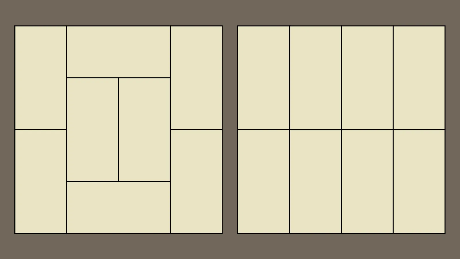
Two traditional tatami layouts. The layout on the left follows the
no-four-corners rule of shūgishiki. The grid layout on the right is a
bushūgishiki, a “layout for sad occasions”.
Shūgishiki tatami arrangements were first considered as combinatorial objects by Kotani in 2001 and gained some attention after Knuth including them in The Art of Computer Programming.
Construction
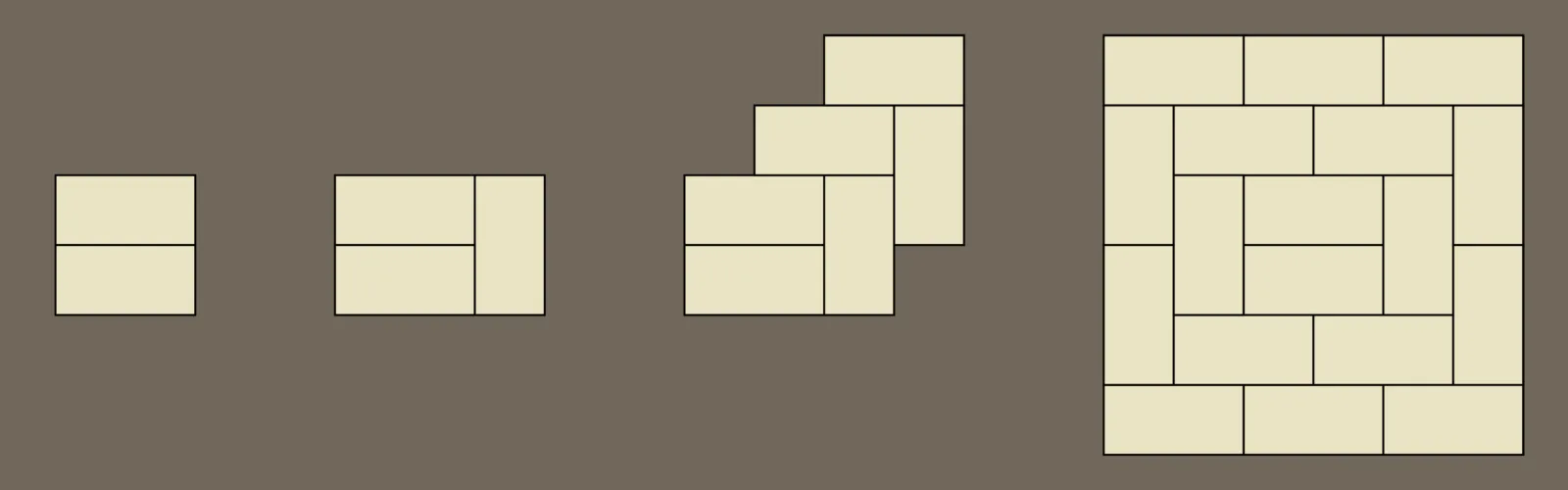
Once you lay down the first couple tatami, you’ll find there aren’t many ways to extend them to a shūgishiki. For example, two side-by-side tatami force the position of all of the surrounding mats until you hit a wall.
Two side-by-side tatami force the arrangement of an entire m×m
square.
This observation can be used to decompose rectangular shūgishiki into
Four-and-a-half tatami rooms can also be found in Japanese homes and tea houses, so naturally mathematicians have also looked into tatami tilings with half-tatami. Alejandro Erickson’s PhD thesis reviews and extends the research into this area. Alejandro has also published a book of puzzles about tatami layouts.
In reality, grid layouts are also used for practical reasons in inns, temples,
and other large gathering halls.
When the Ontario cities of Fort William and Port Arthur amalgamated in 1970, residents voted for a new name for their new city.
The result deserves a place of honour in voting theory textbooks.
I have a new paper with Jing Huang in Graphs and Combinatorics! This was the culmination of my undergraduate research, and shows that a single strategy can be used to solve the monopolar partition problem in all graph classes for which the problem was previously known to be tractable, including line graphs and claw-free graphs.
This research was completed in the summer of 2010, my last undergraduate research term. I am grateful to NSERC for funding my work with a Undergraduate Student Research Award, and to my supervisor and coauthor Jing Huang.
Image Evolution is a very interesting Javascript tool based on Roger Johansson’s Evo-Lisa idea. It uses a genetic algorithm to represent images as a collection of overlapping polygons.
We start from [a set of random] polygons that are invisible. In each optimization step we randomly modify one parameter (like color components or polygon vertices) and check whether such new variant looks more like the original image. If it is, we keep it, and continue to mutate this one instead.
Just feed it an image and hit start, and a random collection of coloured polygons will gradually evolve into a cool abstract rendition of your picture.
Ever wonder why LaTeX doesn’t provide a way for printing the title and author once \maketitle has been issued? I did. So I asked a question on the TeX StackExchange and received an interesting answer. Turns out it’s an artifact of the times when memory was in extremely short supply.
The main reason was “main-memory” back in those days. LaTeX was effectively eating up half of the available space just through macro definitions. So with complicated pages or with some picture environments etc you could hit the limit. So freeing up any bit was essential and you still see traces of this in the code.
I have successfully defended my master’s thesis on graph-transverse matching problems! It considers the computational complexity of deciding whether a given graph admits a matching which covers every copy of a fixed tree or cycle.
The thesis is related to my previous work on cycle-transverse matchings and P4-transverse matchings and, roughly speaking, shows that H-transverse matchings are NP-hard to find when H is a big cycle or tree, and tractable when H is a triangle or a small tree.
I am grateful to NSERC for funding my degree with a Alexander Graham Bell Canada Graduate Scholarship, and to my supervisor Jing Huang.
I defend my thesis in two weeks, but I’ll be prepared for the snake fight portion thanks to McSweeney’s guide:
Do I have to kill the snake?
University guidelines state that you have to “defeat” the snake. There are many ways to accomplish this. Lots of students choose to wrestle the snake. Some construct decoys and elaborate traps to confuse and then ensnare the snake. One student brought a flute and played a song to lull the snake to sleep. Then he threw the snake out a window.
Are the snakes big?
We have lots of different snakes. The quality of your work determines which snake you will fight. The better your thesis is, the smaller the snake will be.
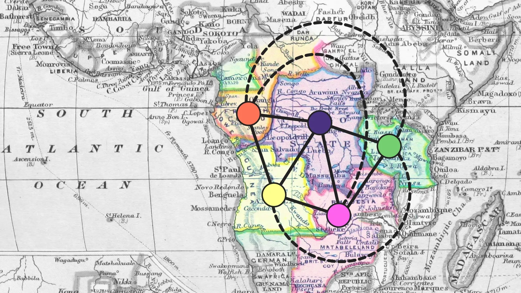
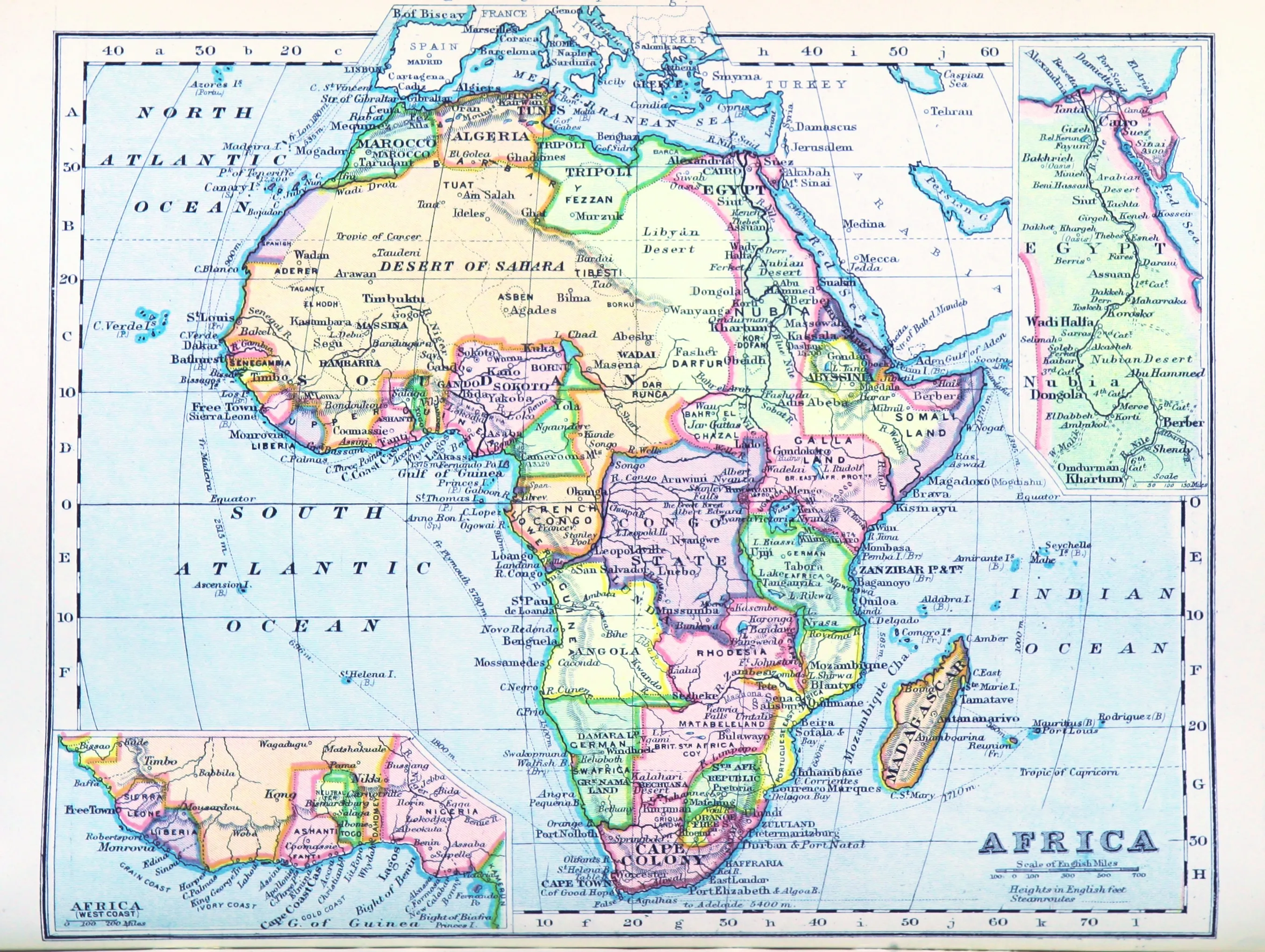
In 1852, then-student Francis Guthrie wondered any if possible map required more than four colours. By the end of the century, Guthrie and his fellow colonists had drawn a map on Africa that needed five.
The Four-Colour Theorem says that, no matter what the borders on your map are, you only need four colours to make sure that neighbouring regions are coloured differently. The theorem doesn’t apply if you let some regions claim other disconnected regions as their own, and in fact the map of European claims on Africa required five colours by the end of the 19th century.
Francis Guthrie, who moved to the South African Cape Colony in 1861, could well have owned a map like the above. Five colours are necessary to properly colour the land that Britain (red), France (orange), Portugal (yellow), Germany (green), and Belgium’s King Leopold II (purple) decided should belong to them.
Five territorities in the center are key to the map colouring:
The boundaries between these colonies separate seven different pairs of empires. Borders between other African colonies account for the other three possible sets of neighbours:
In short, the adjacency graph between these empires was the complete graph K5.
A little while ago, I did some sleuthing to find out the Erdős number of Brian May, astrophysicist and guitarist from Queen. My travels led me to Timeblimp, who threw together three measures of professional collaboration to make a rather fun parlour game. Assuming that the people in your parlour are three kinds of nerds and enjoy long and complicated internet scavenger hunts. Which I am and I do.
The game is to find a well-known person who has published academically, released a song, and been involved in a movie or TV show. Then, you play three versions of Six Degrees of Kevin Bacon: find a series of movies to connect them to prolific actor Kevin Bacon, a series of coauthored papers to connect them to the eccentric mathematician Paul Erdős, and a series of musical collaborations to get to Black Sabbath. Add up all the links and you get the Erdős-Bacon-Sabbath number.
Brian Cox has an Erdős-Bacon-Sabbath number
If anyone has an Erdős-Bacon-Sabbath number, Brian Cox is exactly the sort of person you might expect to have one. The keyboardist, particle physicist, and BBC science presenter is no more than 7+3+3 degrees of separation from the centers of the EBS graph.
Sean from Timeblimp first suggested the possibility of Brian Cox having a well-defined Erdős-Bacon-Sabbath number, but to my knowledge nobody had worked out his Erdős number until now. I managed to find a path of length seven.
The above connections use only papers with three coauthors or fewer. Cox has worked in gigantic collaborations like ATLAS, so it’s quite possible that there might be a shorter path.
Brian Cox — not to be confused with the other Brian Cox — is three degrees of separation from Kevin Bacon through his many TV appearances, including cameos on Doctor Who.
After I published this post, someone brought it to the attention to none other than Brian Cox himself!
The resulting hullabaloo led to the discovery of many other Erdős-Bacon-Sabbath numbers. Eventually, I retired from EBS research after realizing its flaws as a game and as a social construct.
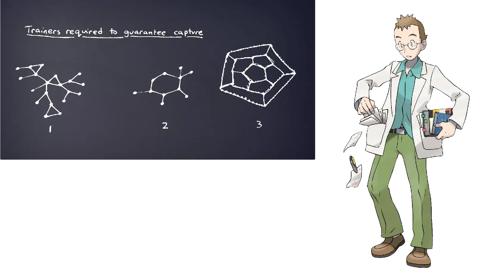
Pokémon Gold and Silver introduced the roaming legendary beasts: three one-of-a-kind Pokémon that move from route to route instead of sticking to a fixed habitat. Catching a roaming Pokémon amounts to winning a graph pursuit game — so what can we learn about it from the latest mathematical results?
To review the Pokémon mechanics, each species can normally be found in a handful of fixed habitats. If you want to catch Abra, you go to Route 24; if you’re looking for Jigglypuff, head to Route 46.
Jigglypuff can always be found on Route 46.
The legendary Entei, Raikou, and Suicune1 are different. There’s only one of each species, each situated on a random route. Each time the player character moves to a new location, the roaming Pokémon each move to a randomly-selected route adjacent to the one they were just on. In graph theory terms, the player and Pokémon are engaged in a pursuit game where the Pokémon’s strategy follows a random walk.
The study of graph pursuit games is a fascinating and active area of research. Classically, researchers have asked how many “cops” it takes to guarantee the capture of an evasive “robber” travelling around a graph. Depending on the graph, many cops might be needed to catch a clever robber; there is a deep open problem about the worst-case cop numbers of large graphs.
Because the graph corresponding to the Pokémon region of Johto contains a long cycle as an isometric subgraph, its cop number is more than one — in other words, it’s possible that a roaming Pokémon could theoretically evade a lone Pokémon trainer forever! Fortunately, the legendary beasts play randomly, not perfectly, so the worst-case scenario doesn’t apply.
A random walk in an arbitrary n-vertex, m-edge graph can be expected to spend deg(v)/(2m) of its time at each location v, and to visit the whole graph after at most roughly 4n3/27 steps. So any trainer who isn’t actively trying to avoid Entei should end up bumping into it eventually — and an intelligent trainer should be able to do much better.
The first place to start is the “greedy” strategy I originally tried as a kid: every time Entei moves, check the map, and move to any route that gets me closer to them. After Entei makes its random move, the distance between us could be unchanged (with Entei’s move offsetting mine), or it could go down by one, or it could go down by two in the lucky 1/Δ chance that Entei moves towards me. If I start at a distance of ℓ steps away from Entei and get lucky ℓ/2 times, I’ll have caught up — so using a negative binomial distribution bound,
E[capture time]≤2Δℓ.
In the grand scheme of things, this isn’t too bad — especially if Δ is low. But it still takes a frustratingly large time for a 12-year-old, and in general it’s possible to do better.
Professor Elm ponders some results and conjectures about graph pursuit games.
Recently, Peter Winkler and Natasha Komarov found a strategy for general graphs which gives a better bound on the expected capture time. Somewhat counterintuitively, it involves aiming for where the robber was — rather than their current location — until the cop is very close to catching him. The Komarov-Winkler strategy has an expected capture time of n+o(n), where n is the number of locations on the map. This is essentially best possible on certain graphs, and is better than the above Δℓ/2 bound when the graph has vertices with large degree.
For graphs without high-degree vertices — like the Pokémon world map — it is possible that a simpler solution could beat the Komarov–Winkler strategy. The problem is: simpler strategies may not be simpler to analyse. In her PhD thesis, Natasha wondered whether a greedy algorithm with random tiebreakers could guarantee n+o(n) expected capture time. It is an open question to find a general bound for the “randomly greedy” strategy’s expected performance that would prove her right.
I’m including Suicune in this list since it roamed in the original Gold and
Silver, but its behaviour is different from the others in Pokémon Crystal,
HeartGold, and SoulSilver.
Dr Robb Fry, one of my professors from my Thompson Rivers University days, passed away earlier this year at far too young an age. Robb was a real character, a great teacher, and a lot of fun to know.
I took my second course in linear algebra with Robb, and it was one of the most entertaining courses of my first two years. While visiting my parents over the holidays, I dug out my course notes — the only full set of notes I ever took in undergrad — so I could share some memorable episodes from my time with him.
Introducing the notation ”∃!”
It means “there exists a unique…” but I always read it like it’s a William Shatner thing. THERE EXISTS!
On terminology
ROBB: An oval…
CLASS: Don’t you mean an ellipse?
ROBB: Yeah, whatever the real term for that is.
On yellow chalk
I’m going to avoid yellow chalk today, because I have a suspicion that one day they’ll find that the stuff that makes it yellow is toxic. That’s going to be someone’s Ph.D. thesis one day, The Toxic Effects of Yellow Chalk, and I don’t want to be part of the study group.
On the kernel (which gets “killed” by a map)
The best bumper sticker I’ve ever seen had a picture of the colonel from KFC with “I am dead.”
On writing
If you’re ever reading a paper, and they say they have to prove a technical lemma, brace yourself for some horrific math.
On stable/invariant sets
I use “invariant” instead of “stable.” A stable set sounds like something for horses. I like horses, mind you, but they shouldn’t be confused with mathematics.
You taught me, inspired me, and motivated me to continue on the path to becoming a mathematician. But more importantly, it was a lot of fun to know you. Thanks, Robb.
Shortly after solving the monopolar partition problem for line graphs, Jing Huang and I realized that our solution could be used to solve the “precoloured” version of the problem, and then further extended to claw-free graphs. Jing presented our result at the French Combinatorial Conference and the proceedings have now been published in Discrete Mathematics.
I’ve published a new paper in the SIAM Journal on Discrete Mathematics! The work is the result of the research term I took as an undergraduate in the summer of 2009. It studies the edge versions of the monopolar and polar partition problems, and presents a linear-time solution to both.
I am grateful to NSERC for funding my work with a Undergraduate Student Research Award, and to my supervisor and coauthor Jing Huang.
Earlier this year, I presented the first results of what would become my master’s thesis at the International Workshop on Combinatorial Algorithms. The paper, coauthored with Jing Huang and Xuding Zhu, has now been published in the LNCS proceedings. It studies the computational complexity of the following problem: in a given graph, is there a matching which breaks all cycles of a given length?
I am grateful to NSERC for funding this research with a Alexander Graham Bell Canada Graduate Scholarship.
I was recently told that European hotels are subject to a reduced VAT rate. They must have a big lobby.
My most recent talk in UVic’s discrete math seminar presented three poetic proofs by Adrian Bondy… and three actual poems summarizing the ideas in each one.
Ore’s Theorem
A red-blue Kn: bluest Hamilton circuit lies fully in G.
Ore’s theorem states:
Let G be a simple graph on n≥3 vertices such that d(u)+d(v)≥n for any nonadjacent u,v. Then G contains a Hamilton cycle.
Bondy’s proof is roughly as follows. Colour the edges of G blue and add red edges to make a complete graph. The complete graph on n≥3 vertices has no shortage of Hamilton cycles, so choose one and label it v1v2…vnv1.
Consider the blue neighbours of v1 on the cycle, and then move one vertex to the right along the cycle so you’re looking at the set
S={vi+1:v1vi∈E(G)}
There are dG(v1) of these vertices, and if v1v2 is red (i.e. v1 and v2 are nonadjacent in G), then the theorem’s hypothesis tells us that
∣S∣=dG(v1)≥n−dG(v2).
Since v2 has only n−1−dG(v2) red neighbours and is not itself in S, that means at least one vertex vi+1∈S is a blue neighbour of v2. We can now replace v1v2 and vivi+1 in the cycle with the two blue edges v1v2 and v2vi+1 to get a Hamilton cycle of Kn with at least one more blue edge than we had before.
We can make the same argument again and again until we have a Hamilton cycle of Kn with no red edges. The cycle being blue means it lies entirely in G, which proves the theorem.
Brooks’ Theorem
Greedily colour, ensuring neighbours follow all except the last.
Choose the last vertex wisely: friend of few or of leaders.
If G is connected and is not an odd cycle or a clique, then χ(G)≤Δ(G).
If G is not regular, Bondy colours it as follows. Let r be a vertex of smaller-than-maximum degree. If we consider the vertices in the reverse order of a depth-first search rooted at r, each vertex other than r has at least one neighbour later in the order and at most d(v)−1 neighbours earlier. Greedily colouring in this order will assign one of the first d(v)≤Δ(v) colours to each v=r, and at least one colour remains available for r since its degree is strictly smaller than Δ(G).
If G is regular, there are a few cases. If it has a cut vertex, we can break the graph into two (non-regular) parts, colour each of them separately, and put them back together. If it has a depth-first tree that branches at some point, then Bondy constructs an ordering similar to the one for the non-regular case: if x has distinct children y,z in the tree, G can be ordered so y and z come first, x comes last, and every other vertex has at least one neighbour later on in the order. A greedy colouring according to this order uses at most Δ(G) colours.
Finally, if G is regular, 2-connected, and all of its depth-first trees are paths, it turns out that G must be a chordless cycle, a clique, or a complete bipartite graph. Since bipartite graphs have χ(G)=2≤Δ(G), the only exceptions to the theorem are odd cycles and cliques.
Vizing’s Theorem
Induction on n. Swap available colours and find SDR.
Vizing’s theorem says:
For any simple graph G, the edge chromatic number χ′(G) is at most Δ(G)+1.
The proof is by induction on the number of vertices; pick a vertex v and start with a (Δ(G)+1)-edge-colouring of G−v.
Ideally, we could just colour the edges around v and extend the edge-colouring to one of G. Those colours would need to be a system of distinct representatives (SDR) for the sets of colours still available at each of the neighbours of v.
If we can’t find a full SDR, then we can still try to colour as many of v‘s edges as possible. Then, if an edge uv is still uncoloured, we can follow a proof of Hall’s Theorem to get a set of coloured edges u1v,u2v,…,ukv such that:
uv can’t be coloured because there are fewer than k+1 total colours among those available at u and u1,u2,…,uk in the colouring of G−v, but
if you un-colour any one of the edges and swap around the colours of the other ones, it would become possible to colour uv.
Note also that
regardless of how we assign Δ(G)+1 colours to edges of G, each vertex will have at least one colour left unused by the edges around it.
The first and third facts put together tell us that some colour (say, blue) is available at two vertices among u and u1,u2,…,uk.
The second fact implies that any colour (e.g. red) still available at v can’t be available at any of the ui, as otherwise we could swap around the colours to colour uv and then use red for uiv.
Look at the subgraph H of G formed by the red and blue edges — it’s made of paths and even cycles. We know that v is incident with a blue edge but not a red one, so it’s the end of a path in H.
We also know that there are two vertices among u,u1,u2,…,uk that are incident with a red edge but not a blue one; those are also ends of paths in H. The paths might be the same as each other, and one might be the same as v‘s path, but the important thing is that we have a red-blue path where at least one of the ends is a neighbour u′ of v and the other end is any vertex other than v.
We can now modify the colouring of G−v to swap red and blue along this path, which frees up red at u′. If u′ is u itself, then we can colour uv red; otherwise, we can uncolour u′v, swap colours around to colour uv, and use red for u′v.
Either way, we’ve shown that the modified colouring of G−v has a larger set of distinct representatives than the original colouring. By repeating this process, we eventually find a colouring of G−v that has a full SDR — and therefore can be extended to a full (Δ(G)+1)-edge-colouring of G.
My Lords, the administration is fully aware of the problem with mice in the Palace of Westminster. I saw one in the Bishops’ Bar only yesterday evening. I do not know whether it was the same one that I saw the day before or a different one; it is always difficult to tell the difference between the various mice that one sees.
The trouble [with reporting mice by telephone] is that when the person at the other end of the helpline goes to check this out, very often the mouse has gone elsewhere.
If you’ve heard of Erdős numbers, Erdős-Bacon numbers, and the fact that Queen lead guitarist Brian May has a PhD, you may have wondered whether Brian May has a well-defined Erdős number.
As a matter of fact, he does! I traced down a collaboration path of length seven through a 1972 paper he published in Nature.
This beats the best previous attempt I found, a path of length eight through a popular science book cowritten by May. It gives him an Erdős-Bacon number of at most 10 (and an Erdős-Bacon-Sabbath number of at most 11).
Did you hear the one about the geology costume contest?